Chapter 1 Loss Data and Insurance Activities
PdfEval = FALSE
A qualitativeThis is a type of variable in which the measurement denotes membership in a set of groups, or categories, or categorical variableA variable whose values are qualitative groups and can have no natural ordering (nominal) or an ordering (ordinal) is one for which the measurement denotes membership in a set of groups, or categories.
Chapter Preview. This book introduces readers to methods of analyzing insurance data. Section 1.1 begins with a discussion of why the use of data is important in the insurance industry. Section 1.2 gives a general overview of the purposes of analyzing insurance data which is reinforced in the Section 1.3 case study. Naturally, there is a huge gap between the broad goals summarized in the overview and a case study application; this gap is covered through the methods and techniques of data analysis covered in the rest of the text.
1.1 Data Driven Insurance Activities
In this section, you learn how to:
- Summarize the importance of insurance to consumers and the economy
- Describe the role that data plays in managing insurance activities
- Identify data generating events associated with the timeline of a typical insurance contract
1.1.1 Nature and Relevance of Insurance
This book introduces the process of using data to make decisions in an insurance context. It does not assume that readers are familiar with insurance but introduces insurance concepts as needed. Insurance is the exchange of a certain amount, known as a premium, for a promise to compensate another party upon the occurrence of an insured event.
If you are new to insurance, then it is probably easiest to think about an insurance policy that covers the contents of an apartment or house that you are renting (known as renters insuranceRenters insurance is an insurance policy that covers the contents of an apartment or house that you are renting.) or the contents and property of a building that is owned by you or a friend (known as homeowners insuranceHomeowners insurance is an insurance policy that covers the contents and property of a building that is owned by you or a friend.). Another common example is automobile insuranceAn insurance policy that covers damage to your vehicle, damage to other vehicles in the accident, as well as medical expenses of those injured in the accident.. In the event of an accident, this policy may cover damage to your vehicle, damage to other vehicles in the accident, as well as medical expenses of those injured in the accident.
One way to think about the nature of insurance is who buys it. Renters, homeowners, and auto insurance are examples of personal insuranceInsurance purchased by a person in that these are policies issued to people. Businesses also buy insurance, such as coverage on their properties, and this is known as commercial insurance. The seller, an insurance company, is also known as an insurer. Even insurance companies need insurance; this is known as reinsuranceInsurance purchased by an insurer.
Another way to think about the nature of insurance is the type of risk being covered. In the U.S., policies such as renters and homeowners are known as property insuranceProperty insurance is a policy that protects the insured against loss or damage to real or personal property. the cause of loss might be fire, lightening, business interruption, loss of rents, glass breakage, tornado, windstorm, hail, water damage, explosion, riot, civil commotion, rain, or damage from aircraft or vehicles. whereas a policy such as auto that covers medical damages to people is known as casualty insuranceCausalty insurance is a form of liability insurance providing coverage for negligent acts and omissions. examples include workers compensation, errors and omissions, fidelity, crime, glass, boiler, and various malpractice coverages.. In the rest of the world, these are both known as non-lifeNon-life insurance is any type of insurance where payments are not based on the death (or survivorship) of a named insured. examples include automobile, homeowners, and so on. also known as property and casualty or general insurance. or general insurance, to distinguish them from life insuranceLife insurance is a contract where the insurer promises to pay upon the death of an insured person. the person being paid is the beneficiary. .
Both life and non-life insurances are important components of the world economy. The The Organization for Economic Cooperation and Development (OECD) (2021) estimates that direct insurance premiums in the OECD (Organization for Economic Cooperation and Development) countries for 2020 was 2,520,220 for life and 2,704,799 for non-life; these figures are in millions of U.S. dollars. The total represents 9.447% of the OECD gross domestic product (GDP). As examples, premiums accounted for 30.9% of GDP in Luxembourg and 17.0% of GDP in Chinese Taipei (the two highest in the study) and represented 12.5% of GDP in the United States. Both life and non-life insurances represent important economic activities.
Insurance affects the financial livelihoods of many and, by almost any measure, insurance is a major economic activity. As noted earlier, on a global level insurance premiums comprised nearly 9.5% of GDP in 2020. On a personal level, almost everyone owning a home has insurance to protect themselves in the event of a fire, hailstorm, or some other calamitous event. Almost every country requires insurance for those driving a car. In sum, insurance plays an important role in the economies of nations and the lives of individuals.
1.1.2 Why Data Driven?
Insurance is a data-driven industry. Like all major corporations and organizations, insurers use data when trying to decide how much to pay employees, how many employees to retain, how to market their services and products, how to forecast financial trends, and so on. These represent general areas of activities that are not specific to the insurance industry. Although each industry has its own data nuances and needs, the collection, analysis and use of data is an activity shared by all, from the internet giants to a small business, by public and governmental organizations, and is not specific to the insurance industry. You will find that the data collection and analysis methods and tools introduced in this text are relevant for all.
In any data-driven industry, deriving and extracting information from data is critical. Making data-driven business decisions has been described as business analytics, business intelligence, and data science. These terms, among others, are sometimes used interchangeably and sometimes refer to distinct applications. Business intelligence may focus on processes of collecting data, often through databases and data warehouses, whereas business analytics utilizes tools and methods for statistical analyses of data. In contrast to these two terms that emphasize business applications, the term data science can encompass broader data related applications in many scientific domains. For our purposes, we use the term analyticsAnalytics is the process of using data to make decisions. to refer to the process of using data to make decisions. This process involves gathering data, understanding concepts and models of uncertainty, making general inferences, and communicating results. Chapter 2 describes data analytics in further detail.
When introducing methods in this text, we focus on loss data that arise from, or are related to, obligations in insurance contracts. This could be the amount of damage to one’s apartment under a renter’s insurance agreement, the amount needed to compensate someone that you hurt in a driving accident, and the like. We call such payments an insurance claimAn insurance claim is the compensation provided by the insurer for incurred hurt, loss, or damage that is covered by the policy.. With this focus, we are able to introduce and directly use generally applicable statistical tools and techniques.
1.1.3 Insurance Processes
Yet another way to think about the nature of insurance is by the duration of an insurance contract, known as the termThe duration of an insurance contract. This text will focus on short-term insurance contracts. By short-term, we mean contracts where the insurance coverage is typically provided for a year or six months. Most non-life commercial and personal contracts are for a year so that is our default duration. An important exception is U.S. auto policies that are often six months in length.
In contrast, we typically think of life insurance as a long-term contract where the default is to have a multi-year contract. For example, if a person 25 years old purchases a whole life policy that pays upon death of the insured and that person does not die until age 100, then the contract is in force for 75 years.
There are other important differences between life and non-life products. In life insurance, the benefit amount is often stipulated in the contract provisions. In contrast, most non-life contracts provide for compensation of insured losses which are unknown before the accident. (There are usually limits placed on the compensation amounts.) In a life insurance contract that stretches over many years, the time value of money plays a prominent role. In a non-life contract, the random amount of compensation takes priority.
In both life and non-life insurances, the frequency of claims is very important. For many life insurance contracts, the insured event (such as death) happens only once. In contrast, for non-life insurances such as automobile, it is common for individuals (especially young male drivers) to get into more than one accident during a year. So, our models need to reflect this observation; we introduce different frequency models that you may also see when studying life insurance.
For short-term insurance, the framework of the probabilistic model is straightforward. We think of a one-period model (the period length, e.g., one year, will be specified in the situation).
- At the beginning of the period, the insured pays the insurer a known premium that is agreed upon by both parties to the contract.
- At the end of the period, the insurer reimburses the insured for a (possibly multivariate) random loss.
This framework will be developed as we proceed; but we first focus on integrating this framework with concerns about how the data may arise. From an insurer’s viewpoint, contracts may be only for a year but they tend to be renewed. Moreover, payments arising from claims during the year may extend well beyond a single year. One way to describe the data arising from operations of an insurance company is to use a timeline granular approach. A process approach provides an overall view of the events occurring during the life of an insurance contract, and their nature – random or planned, loss events (claims) and contract changes events, and so forth. In this micro oriented view, we can think about what happens to a contract at various stages of its existence.
Figure 1.1 traces a timeline of a typical insurance contract. Throughout the life of the contract, the company regularly processes events such as premium collection and valuation, described in Section 1.2; these are marked with an x on the timeline. Non-regular and unanticipated events also occur. To illustrate, \(\mathrm{t}_2\) and \(\mathrm{t}_4\) mark the event of an insurance claim (some contracts, such as life insurance, can have only a single claim). Times \(\mathrm{t}_3\) and \(\mathrm{t}_5\) mark events when a policyholder wishes to alter certain contract features, such as the choice of a deductibleA deductible is a parameter specified in the contract. typically, losses below the deductible are paid by the policyholder whereas losses in excess of the deductible are the insurer’s responsibility (subject to policy limits and coninsurance). or the amount of coverage. From a company perspective, one can even think about the contract initiation (arrival, time \(\mathrm{t}_1\)) and contract termination (departure, time \(\mathrm{t}_6\)) as uncertain events. (Alternatively, for some purposes, you may condition on these events and treat them as certain.)
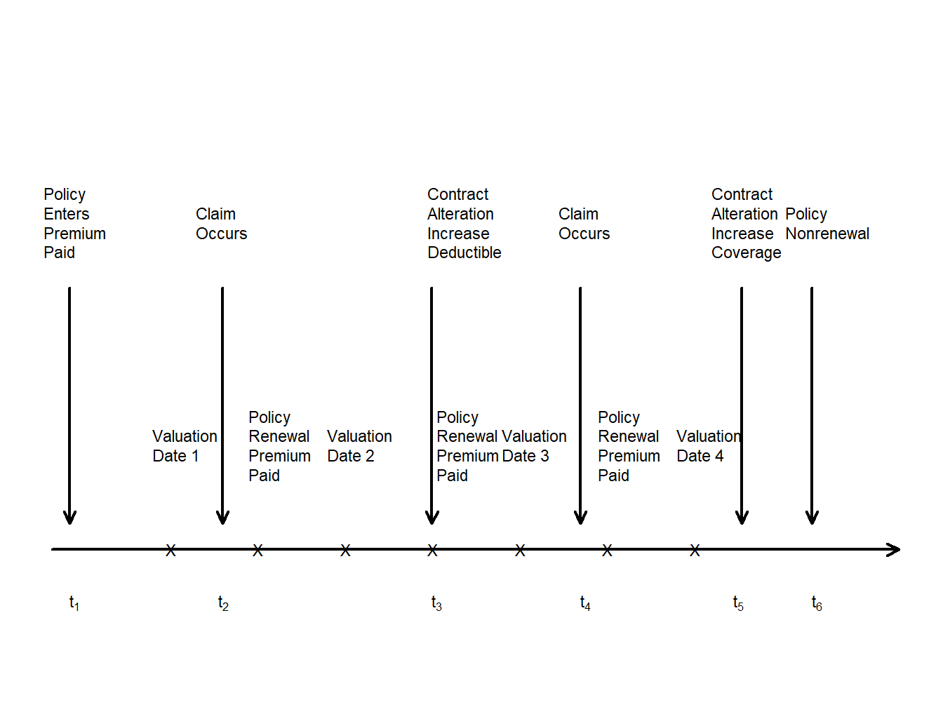
Figure 1.1: Timeline of a Typical Insurance Policy. Arrows mark the occurrences of random events. Each x marks the time of scheduled events that are typically non-random.
Show Quiz Solution
1.2 Insurance Company Operations
In this section, you learn how to:
- Describe five major operational areas of insurance companies.
- Identify the role of data and analytics opportunities within each operational area.
Armed with insurance data, the end goal is to use data to make decisions. We will learn more about methods of analyzing and extrapolating data in future chapters. To begin, let us think about why we want to do the analysis. We take the insurance company’s viewpoint (not the insured person) and introduce ways of bringing money in, paying it out, managing costs, and making sure that we have enough money to meet obligations. The emphasis is on insurance-specific operations rather than on general business activities such as advertising, marketing, and human resources management.
Specifically, in many insurance companies, it is customary to aggregate detailed insurance processes into larger operational units; many companies use these functional areas to segregate employee activities and areas of responsibilities. Actuaries, other financial analysts, and insurance regulators work within these units and use data for the following activities:
- Initiating Insurance. At this stage, the company makes a decision as to whether or not to take on a risk (the underwritingUnderwriting is the process where the company makes a decision as to whether or not to take on a risk. stage) and assign an appropriate premium (or rate). Insurance analytics has its actuarial roots in ratemaking, where analysts seek to determine the right price for the right risk.
- Renewing Insurance. Many contracts, particularly in general insurance, have relatively short durations such as 6 months or a year. Although there is an implicit expectation that such contracts will be renewed, the insurer has the opportunity to decline coverage and to adjust the premium. Analytics is also used at this policy renewal stage where the goal is to retain profitable customers.
- Claims Management. Analytics has long been used in (1) detecting and preventing claims fraud, (2) managing claim costs, including identifying the appropriate support for claims handling expenses, as well as (3) understanding excess layers for reinsurance and retention.
- Loss Reserving. Analytic tools are used to provide management with an appropriate estimate of future obligations and to quantify the uncertainty of those estimates.
- Solvency and Capital Allocation. Deciding on the requisite amount of capital and on ways of allocating capital among alternative investments are also important analytics activities. Companies must understand how much capital is needed so that they have sufficient flow of cash available to meet their obligations at the times they are expected to materialize (solvency). This is an important question that concerns not only company managers but also customers, company shareholders, regulatory authorities, as well as the public at large. Related to issues of how much capital is the question of how to allocate capital to differing financial projects, typically to maximize an investor’s return. Although this question can arise at several levels, insurance companies are typically concerned with how to allocate capital to different lines of business within a firm and to different subsidiaries of a parent firm.
Although data represent a critical component of solvency and capital allocation, other components including the local and global economic framework, the financial investments environment, and quite specific requirements according to the regulatory environment of the day, are also important. Because of the background needed to address these components, we do not address solvency, capital allocation, and regulation issues in this text.
Nonetheless, for all operating functions, we emphasize that analytics in the insurance industry is not an exercise that a small group of analysts can do by themselves. It requires an insurer to make significant investments in their information technology, marketing, underwriting, and actuarial functions. As these areas represent the primary end goals of the analysis of data, additional background on each operational unit is provided in the following subsections.
1.2.1 Initiating Insurance
Setting the price of an insurance product can be a perplexing problem. This is in contrast to other industries such as manufacturing where the cost of a product is (relatively) known and provides a benchmark for assessing a market demand price. Similarly, in other areas of financial services, market prices are available and provide the basis for a market-consistent pricing structure of products. However, for many lines of insurance, the cost of a product is uncertain and market prices are unavailable. Expectations of the random cost is a reasonable place to start for a price. (If you have studied finance, then you will recall that an expectation is the optimal price for a risk-neutral insurer.) It has been traditional in insurance pricing to begin with the expected cost. Insurers then add margins to this, to account for the product’s riskiness, expenses incurred in servicing the product, and an allowance for profit/surplus of the company.
Use of expected costs as a foundation for pricing is prevalent in some lines of the insurance business. These include automobile and homeowners insurance. For these lines, analytics has served to sharpen the market by making the calculation of the product’s expected cost more precise. The increasing availability of the internet to consumers has also promoted transparency in pricing; in today’s marketplace, consumers have ready access to competing quotes from a host of insurers. Insurers seek to increase their market share by refining their risk classificationRisk classification is the process of grouping policyholders into categories, or classes, where each insured in the class has a risk profile that is similar to others in the class. systems, thus achieving a better approximation of the products’ prices and enabling cream-skimming underwriting strategies (“cream-skimming” is a phrase used when the insurer underwrites only the best risks). Surveys (e.g., Earnix (2013)) indicate that pricing is the most common use of analytics among insurers.
Underwriting, the process of classifying risks into homogeneous categories and assigning policyholders to these categories, lies at the core of ratemaking. Policyholders within a class (category) have similar risk profiles and so are charged the same insurance price. This is the concept of an actuarially fair premium; it is fair to charge different rates to policyholders only if they can be separated by identifiable risk factors. An early article, Two Studies in Automobile Insurance Ratemaking (Bailey and LeRoy 1960), provided a catalyst to the acceptance of analytic methods in the insurance industry. This paper addresses the problem of classification ratemaking. It describes an example of automobile insurance that has five use classes cross-classified with four merit rating classes. At that time, the contribution to premiums for use and merit rating classes were determined independently of each other. Thinking about the interacting effects of different classification variables is a more difficult problem.
When the risk is initially obtained, the insurer’s obligations can be managed by imposing contract parameters that modify contract payouts. Chapter 4 describes common modifications including coinsuranceCoinsurance is an arrangement whereby the insured and insurer share the covered losses. typically, a coinsurance parameter specified means that both parties receive a proportional share, e.g., 50%, of the loss., deductibles and policy upper limits.
1.2.2 Renewing Insurance
Insurance is a type of financial service and, like many service contracts, insurance coverage is often agreed upon for a limited time period at which time coverage commitments are complete. Particularly for general insurance, the need for coverage continues and so efforts are made to issue a new contract providing similar coverage when the existing contract comes to the end of its term. This is called policy renewal. Renewal issues can also arise in life insurance, e.g., term (temporary) life insurance. At the same time other contracts, such as life annuities, terminate upon the insured’s death and so issues of renewability are irrelevant.
In the absence of legal restrictions, at renewal the insurer has the opportunity to:
- accept or decline to underwrite the risk; and
- determine a new premium, possibly in conjunction with a new classification of the risk.
Risk classification and rating at renewal is based on two types of information. First, at the initial stage, the insurer has available many rating variables upon which decisions can be made. Many variables are not likely to change, e.g., sex, whereas others are likely to change, e.g., age, and still others may or may not change, e.g., credit score. Second, unlike the initial stage, at renewal the insurer has available a history of policyholder’s loss experience, and this history can provide insights into the policyholder that are not available from rating variables. Modifying premiums with claims history is known as experience rating, also sometimes referred to as merit rating.
Experience rating methods are either applied retrospectively or prospectively. With retrospective methods, a refund of a portion of the premium is provided to the policyholder in the event of favorable (to the insurer) experience. Retrospective premiumsThe process of determining the cost of an insurance policy based on the actual loss experience determined as an adjustment to the initial premium payment. are common in life insurance arrangements (where policyholders earn dividendsA dividend is the refund of a portion of the premium paid by the insured from insurer surplus. in the U.S., bonuses in the U.K., and profit sharing in Israeli term life coverage). In general insurance, prospective methods are more common, where favorable insured experience is rewarded through a lower renewal premium.
Claims history can provide information about a policyholder’s risk appetite. For example, in personal lines it is common to use a variable to indicate whether or not a claim has occurred in the last three years. As another example, in a commercial line such as worker’s compensation, one may look to a policyholder’s average claim frequency or severity over the last three years. Claims history can reveal information that is otherwise hidden (to the insurer) about the policyholder.
1.2.3 Claims and Product Management
In some of types of insurance, the process of paying claims for insured events is relatively straightforward. For example, in life insurance, a simple death certificate is all that is needed to pay the benefit amount as provided in the contract. However, in non-life areas such as property and casualty insurance, the process can be much more complex. Think about a relatively simple insured event such as an automobile accident. Here, it is often required to determine which party is at fault and then one needs to assess damage to all of the vehicles and people involved in the incident, both insured and non-insured. Further, the expenses incurred in assessing the damages must be assessed, and so forth. The process of determining coverage, legal liability, and settling claims is known as claims adjustmentClaims adjustment is the process of determining coverage, legal liability, and settling claims..
Insurance managers sometimes use the phrase claims leakageClaims leakage respresents money lost through claims management inefficiencies. to mean dollars lost through claims management inefficiencies. There are many ways in which analytics can help manage the claims process, c.f., Gorman and Swenson (2013). Historically, the most important has been fraud detection. The claim adjusting process involves reducing information asymmetry (the claimant knows what happened; the company knows some of what happened). Mitigating fraud is an important part of the claims management process.
Fraud detection is only one aspect of managing claims. More broadly, one can think about claims management as consisting of the following components:
- Claims triaging. Just as in the medical world, early identification and appropriate handling of high cost claims (patients, in the medical world), can lead to dramatic savings. For example, in workers compensation, insurers look to achieve early identification of those claims that run the risk of high medical costs and a long payout period. Early intervention into these cases could give insurers more control over the handling of the claim, the medical treatment, and the overall costs with an earlier return-to-work.
- Claims processing. The goal is to use analytics to identify routine situations that are anticipated to have small payouts. More complex situations may require more experienced adjusters and legal assistance to appropriately handle claims with high potential payouts.
- Adjustment decisions. Once a complex claim has been identified and assigned to an adjusterAn adjuster is a person who investigates claims and recommends settlement options based on estimates of damage and insurance policies held., analytic driven routines can be established to aid subsequent decision-making processes. Such processes can also be helpful for adjusters in developing case reserves, an estimate of the insurer’s future liability. This is an important input to the insurer’s loss reserves, described in Section 1.2.4.
In addition to the insured’s reimbursement for losses, the insurer also needs to be concerned with another source of revenue outflow, expenses. Loss adjustment expensesLoss adjustment expenses are costs to the insurer that are directly attributable to settling a claims. for example, the cost of an adjuster is someone who assess the claim cost or a lawyer who becomes involve in settling an insurer’s legal obligation on a claim are part of an insurer’s cost of managing claims. Analytics can be used to reduce expenses directly related to claims handling (allocatedAllocated loss adjustment expenses, sometimes known by the acronym alea, are costs that can be directly attributed to settling a claim; for example, the cost of an adjuster) as well as general staff time for overseeing the claims processes (unallocatedUnallocated loss adjustment expenses are costs that can only be indirectly attributed to claim settlement; for example, the cost of an office to support claims staff). The insurance industry has high operating costs relative to other portions of the financial services sectors.
In addition to claims payments, there are many other ways in which insurers use data to manage their products. We have already discussed the need for analytics in underwriting, that is, risk classification at the initial acquisition and renewal stages. Insurers are also interested in which policyholders elect to renew their contracts and, as with other products, monitor customer loyalty.
Analytics can also be used to manage the portfolio, or collection, of risks that an insurer has acquired. As described in Chapter 13, after the contract has been agreed upon with an insured, the insurer may still modify its net obligation by entering into a reinsurance agreement. This type of agreement is with a reinsurer, an insurer of an insurer. It is common for insurance companies to purchase insurance on its portfolio of risks to gain protection from unusual events, just as people and other companies do.
1.2.4 Loss Reserving
An important feature that distinguishes insurance from other sectors of the economy is the timing of the exchange of considerations. In manufacturing, payments for goods are typically made at the time of a transaction. In contrast, for insurance, money received from a customer occurs in advance of benefits or services; these are rendered at a later date if the insured event occurs. This leads to the need to hold a reservoir of wealth to meet future obligations in respect to obligations made, and to gain the trust of the insureds that the company will be able to fulfill its commitments. The size of this reservoir of wealth, and the importance of ensuring its adequacy, is a major concern for the insurance industry.
Setting aside money for unpaid claims is known as loss reservingA loss reserve is an estimate of liability indicating the amount the insurer expects to pay for claims that have not yet been realized. this includes losses incurred but not yet reported (ibnr) and those claims that have been reported claims that haven’t been paid (known by the acronym rbns for reported but not settled).; in some jurisdictions, reserves are also known as technical provisions. We saw in Figure 1.1 several times at which a company summarizes its financial position; these times are known as valuation dates. Claims that arise prior to valuation dates have either been paid, are in the process of being paid, or are about to be paid; claims in the future of these valuation dates are unknown. A company must estimate these outstanding liabilities when determining its financial strength. Accurately determining loss reserves is important to insurers for many reasons.
- Loss reserves represent an anticipated claim that the insurer owes its customers. Under-reserving may result in a failure to meet claim liabilities. Conversely, an insurer with excessive reserves may present a conservative estimate of surplus and thus portray a weaker financial position than it truly has.
- Reserves provide an estimate for the unpaid cost of insurance that can be used for pricing contracts.
- Loss reserving is required by laws and regulations. The public has a strong interest in the financial strength and solvency of insurers.
- In addition to regulators, other stakeholders such as insurance company management, investors, and customers make decisions that depend on company loss reserves. Whereas regulators and customers appreciate conservative estimates of unpaid claims, managers and investors seek more unbiased estimates to represent the true financial health of the company.
Loss reserving is a topic where there are substantive differences between life and general (also known as property and casualty, or non-life) insurance. In life insurance, the severity (amount of loss) is often not a source of uncertainty as payouts are specified in the contract. The frequency, driven by mortality of the insured, is a concern. However, because of the lengthy time for settlement of life insurance contracts, the time value of money uncertainty as measured from issue to date of payment can dominate frequency concerns. For example, for an insured who purchases a life contract at age 20, it would not be unusual for the contract to still be open in 60 years time, when the insured celebrates his or her 80th birthday. See, for example, Bowers et al. (1986) or Dickson, Hardy, and Waters (2013) for introductions to reserving for life insurance. In contrast, for most lines of non-life business, severity is a major source of uncertainty and contract durations tend to be shorter.
Show Quiz Solution
1.3 Case Study: Wisconsin Property Fund
In this section, we use the Wisconsin Property Fund as a case study. You learn how to:
- Describe how data generating events can produce data of interest to insurance analysts.
- Produce relevant summary statistics for each variable.
- Describe how these summary statistics can be used in each of the major operational areas of an insurance company.
Let us illustrate the kind of data under consideration and the goals that we wish to achieve by examining the Local Government Property Insurance Fund (LGPIF), an insurance pool administered by the Wisconsin Office of the Insurance Commissioner. The LGPIF was established to provide property insurance for local government entities that include counties, cities, towns, villages, school districts, and library boards. The fund insures local government property such as government buildings, schools, libraries, and motor vehicles. It covers all property losses except those resulting from flood, earthquake, wear and tear, extremes in temperature, mold, war, nuclear reactions, and embezzlement or theft by an employee.
The fund covers over a thousand local government entities who pay approximately 25 million dollars in premiums each year and receive insurance coverage of about 75 billion. State government buildings are not covered; the LGPIF is for local government entities that have separate budgetary responsibilities and who need insurance to moderate the budget effects of uncertain insurable events. Coverage for local government property has been made available by the State of Wisconsin since 1911, thus providing a wealth of historical data.
In this illustration, we restrict consideration to claims from coverage of building and contents; we do not consider claims from motor vehicles and specialized equipment owned by local entities (such as snow plowing machines). We also consider only claims that are closed, with obligations fully met.
1.3.1 Fund Claims Variables: Frequency and Severity
At a fundamental level, insurance companies accept premiums in exchange for promises to compensate a policyholder upon the occurrence of an insured event. IndemnificationIndemnification is the compensation provided by the insurer. is the compensation provided by the insurer for incurred hurt, loss, or damage that is covered by the policy. This compensation is also known as a claim. The extent of the payout, known as the severity, is a key financial expenditure for an insurer.
In terms of money outgo to customers, an insurer is indifferent to having ten claims of 100 when compared to one claim of 1,000. Nonetheless, it is common for insurers to study how often claims arise, known as the frequency of claims. The frequency is important for expenses, but it also influences contractual parameters (such as deductibles and policy limits that are described later) that are written to limit amounts paid for each occurrence of an insured event. Frequency is routinely monitored by insurance regulators and can be a key driver in the overall indemnification obligation of the insurer. We shall consider the frequency and severity as the two main claim variables that we wish to understand, model, and manage.
To illustrate, in 2010 there were 1,110 policyholders in the property fund who experienced a total of 1,377 claims. Table 1.1 shows the distribution. Almost two-thirds (0.637) of the policyholders did not have any claims and an additional 18.8% had only one claim. The remaining 17.5% (=1 - 0.637 - 0.188) had more than one claim; the policyholder with the highest number recorded 239 claims. The average number of claims for this sample was 1.24 (=1377/1110).
| Number | 0 | 1 | 2 | 3 | 4 | 5 | 6 | 7 | 8 | 9 or more | Sum |
| Policies | 707 | 209 | 86 | 40 | 18 | 12 | 9 | 4 | 6 | 19 | 1110 |
| Claims | 0 | 209 | 172 | 120 | 72 | 60 | 54 | 28 | 48 | 614 | 1377 |
| Proportion | 0.637 | 0.188 | 0.077 | 0.036 | 0.016 | 0.011 | 0.008 | 0.004 | 0.005 | 0.017 | 1 |
R Code for Frequency Table
For the severity distribution, a common approach is to examine the distribution of the sample of 1,377 claims. However, another common approach is to examine the distribution of the average claims of those policyholders with claims. In our 2010 sample, there were 403 (=1110-707) such policyholders. For 209 of these policyholders with one claim, the average claim equals the only claim they experienced. For the policyholder with highest frequency, the average claim is an average over 239 separately reported claim events.
Table 1.2 summarizes the sample distribution of average severities from the 403 policyholders who made a claim; it shows that the average claim amount was 56,330 (all amounts are in U.S. Dollars). However, the average gives only a limited look at the distribution. More information can be gleaned from the summary statistics which show a very large claim in the amount of 12,920,000. Figure 1.2 provides further information about the distribution of sample claims, showing a distribution that is dominated by this single large claim so that the histogram is not very helpful. Even when removing the large claim, you will find a distribution that is skewed to the right. A generally accepted technique is to work with claims in logarithmic units especially for graphical purposes; the corresponding figure in the right-hand panel is much easier to interpret.
| Minimum | First Quartile | Median | Mean | Third Quartile | Maximum |
|---|---|---|---|---|---|
| 167 | 2,226 | 4,951 | 56,332 | 11,900 | 12,922,218 |
R Code for Average Severity Distribution
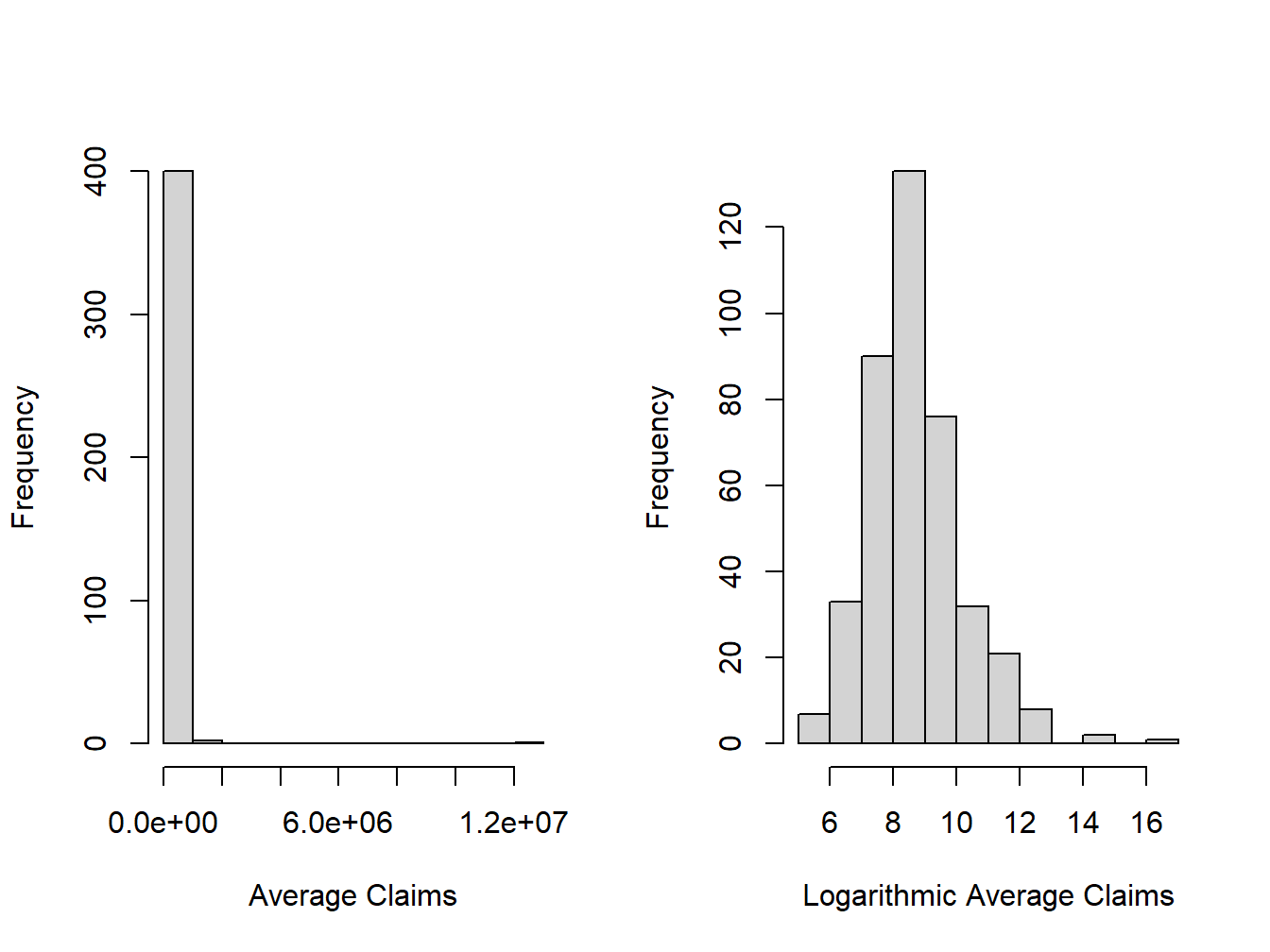
Figure 1.2: Distribution of Positive Average Severities
R Code for Severity Distribution Table and Figures
1.3.2 Fund Rating Variables
Developing models to represent and manage the two outcome variables, frequency and severity, is the focus of the early chapters of this text. However, when actuaries and other financial analysts use those models, they do so in the context of external variables. In general statistical terminology, one might call these explanatory or predictor variables; there are many other names in statistics, economics, psychology, and other disciplines. Because of our insurance focus, we call them rating variablesRating variables are the components of an insurance pricing formula. they can include numeric variables (like values, revenue, or area) and classification variables (like location, type of vehicle, or type of occupancy.) as they are useful in setting insurance rates and premiums.
We earlier considered observations from a sample of 1,110 policyholders which may seem like a lot. However, as we will see in our forthcoming applications, because of the preponderance of zeros and the skewed nature of claims, actuaries typically yearn for more data. One common approach that we adopt here is to examine outcomes from multiple years, thus increasing the sample size. We will discuss the strengths and limitations of this strategy later but, at this juncture, we just wish to show the reader how it works.
Specifically, Table 1.3 shows that we now consider policies over five years of data, 2006, …, 2010, inclusive. The data begins in 2006 because there was a shift in claim coding in 2005 so that comparisons with earlier years are not helpful. To mitigate the effect of open claims, we consider policy years prior to 2011. An open claim means that not all of the obligations for the claim are known at the time of the analysis; for some claims, such an injury to a person in an auto accident or in the workplace, it can take years before costs are fully known.
| Year | Average Frequency | Average Severity | Average | Number of Policyholders |
|---|---|---|---|---|
| 2006 | 0.951 | 9,695 | 32,498,186 | 1,154 |
| 2007 | 1.167 | 6,544 | 35,275,949 | 1,138 |
| 2008 | 0.974 | 5,311 | 37,267,485 | 1,125 |
| 2009 | 1.219 | 4,572 | 40,355,382 | 1,112 |
| 2010 | 1.241 | 20,452 | 41,242,070 | 1,110 |
R Code for Claims Summary by Policyholder
Table 1.3 shows that the average claim varies over time, especially with the high 2010 value (that we saw was due to a single large claim)1. The total number of policyholders is steadily declining and, conversely, the coverage is steadily increasing. The coverage variable is the amount of coverage of the property and contents. Roughly, you can think of it as the maximum possible payout of the insurer. For our immediate purposes, the coverage is our first rating variable. Other things being equal, we would expect that policyholders with larger coverage have larger claims. We will make this vague idea much more precise as we proceed, and also justify this expectation with data.
For a different look at the 2006-2010 data, Table 1.4 summarizes the distribution of our two outcomes, frequency and claims amount. In each case, the average exceeds the median, suggesting that the two distributions are right-skewed. In addition, the table summarizes our continuous rating variables, coverage and deductible amount. The table also suggests that these variables also have right-skewed distributions.
| Minimum | Median | Average | Maximum | |
|---|---|---|---|---|
| Claim Frequency | 0 | 0 | 1.109 | 263 |
| Claim Severity | 0 | 0 | 9,292 | 12,922,218 |
| Deductible | 500 | 1,000 | 3,365 | 100,000 |
| Coverage (000’s) | 8.937 | 11,354 | 37,281 | 2,444,797 |
R Code for Summary of Claim Frequency and Severity, Deductibles, and Coverages
Table 1.5 describes the rating variables considered in this chapter. Hopefully, these are variables that you think might naturally be related to claims outcomes. You can learn more about them in Frees, Lee, and Yang (2016b). To handle the skewness, we henceforth focus on logarithmic transformations of coverage and deductibles.
Table 1.5. Description of Rating Variables
\[{\small \begin{matrix} \begin{array}{ l | l} \hline Variable & Description \\ \hline \text{EntityType} & \text{Categorical variable that is one of six types: (Village, City,} \\ & ~~~~ \text{County, Misc, School, or Town)} \\ \text{LnCoverage} & \text{Total building and content coverage, in logarithmic millions of dollars}\\ \text{LnDeduct} & \text{Deductible, in logarithmic dollars} \\ \text{AlarmCredit} & \text{Categorical variable that is one of four types: (0, 5, 10, or 15)} \\ & ~~~~ \text{for automatic smoke alarms in main rooms} \\ \text{NoClaimCredit} & \text{Binary variable to indicate no claims in the past two years} \\ \text{Fire5 } & \text{Binary variable to indicate the fire class is below 5} \\ & ~~~~ \text{(The range of fire class is 1 to 10)} \\ \hline \end{array} \end{matrix}}\]
For the alarm credit variable, a zero means that no automatic smoke alarms exist in any of the main rooms. In the same way, a 5 means they exist in some of the main rooms and a 10 means they exist in all of the main rooms. At the 15 level, facilities are monitored on a 24 hours per day, 7 days per week basis by a police, fire, or security company. A fire rating is a similar type of score. It reflects how prepared a community and area is for fires. While it mainly focuses on the local fire departments and water supply, there are other factors that contribute to an area’s score. This rating is used to determine how likely it is for a fire to do severe damage before help arrives with 1 being the best and 10 the worst.
To get a sense of the relationship between the non-continuous rating variables and claims, Table 1.6 relates the claims outcomes to these categorical variables. Table 1.6 suggests substantial variation in the claim frequency and average severity of the claims by entity type. It also demonstrates higher frequency and severity for the \({\tt Fire5}\) variable and the reverse for the \({\tt NoClaimCredit}\) variable. The relationship for the \({\tt Fire5}\) variable is counter-intuitive in that one would expect lower claim amounts for those policyholders in areas with better public protection (when the protection code is five or less). Naturally, there are other variables that influence this relationship. We will see that these background variables are accounted for in the subsequent multivariate regression analysis, which yields an intuitive, appealing (negative) sign for the \({\tt Fire5}\) variable.
| Number of Policies | Claim Frequency | Average Severity | |
|---|---|---|---|
| Village | 1,341 | 0.452 | 10,645 |
| City | 793 | 1.941 | 16,924 |
| County | 328 | 4.899 | 15,453 |
| Misc | 609 | 0.186 | 43,036 |
| School | 1,597 | 1.434 | 64,346 |
| Town | 971 | 0.103 | 19,831 |
| Fire5–No | 2,508 | 0.502 | 13,935 |
| Fire5–Yes | 3,131 | 1.596 | 41,421 |
| NoClaimCredit–No | 3,786 | 1.501 | 31,365 |
| NoClaimCredit–Yes | 1,853 | 0.31 | 30,499 |
| Total | 5,639 | 1.109 | 31,206 |
R Code for Claims Summary by Entity Type, Fire Class, and No Claim Credit
Tables 1.7 and 1.8 show the claims experience by alarm credit. It underscores the difficulty of examining variables individually. For example, when looking at the experience for all entities, we see that policyholders with no alarm credit have on average lower frequency and severity than policyholders with the highest (15%, with 24/7 monitoring by a fire station or security company) alarm credit. In particular, when we look at the entity type School, the frequency is 0.422 and the severity 25,523 for no alarm credit, whereas for the highest alarm level it is 2.008 and 85,140, respectively. This may simply imply that entities with more claims are the ones that are likely to have an alarm system. Summary tables do not examine multivariate effects; for example, Table 1.6 ignores the effect of size (as we measure through coverage amounts) that affect claims.
| AC0 Claim Frequency | AC0 Avg. Severity | AC0 Num. Policies | AC5 Claim Frequency | AC5 Avg. Severity | AC5 Num. Policies | |
|---|---|---|---|---|---|---|
| Village | 0.326 | 11,078 | 829 | 0.278 | 8,086 | 54 |
| City | 0.893 | 7,576 | 244 | 2.077 | 4,150 | 13 |
| County | 2.14 | 16,013 | 50 | 0 | 0 | 1 |
| Misc | 0.117 | 15,122 | 386 | 0.278 | 13,064 | 18 |
| School | 0.422 | 25,523 | 294 | 0.41 | 14,575 | 122 |
| Town | 0.083 | 25,257 | 808 | 0.194 | 3,937 | 31 |
| Total | 0.318 | 15,118 | 2611 | 0.431 | 10,762 | 239 |
| AC10 Claim Frequency | AC10 Avg. Severity | AC10 Num. Policies | AC15 Claim Frequency | AC15 Avg. Severity | AC15 Num. Policies | |
|---|---|---|---|---|---|---|
| Village | 0.5 | 8,792 | 50 | 0.725 | 10,544 | 408 |
| City | 1.258 | 8,625 | 31 | 2.485 | 20,470 | 505 |
| County | 2.125 | 11,688 | 8 | 5.513 | 15,476 | 269 |
| Misc | 0.077 | 3,923 | 26 | 0.341 | 87,021 | 179 |
| School | 0.488 | 11,597 | 168 | 2.008 | 85,140 | 1013 |
| Town | 0.091 | 2,338 | 44 | 0.261 | 9,490 | 88 |
| Total | 0.517 | 10,194 | 327 | 2.093 | 41,458 | 2462 |
R Code for Claims Summary by Entity Type, Fire Class, and No Claim Credit
We will learn more about modeling count data in the Chapter 3 and about severity data in Chapters 4 and 7.
1.3.3 Fund Operations
We have now seen distributions of the Fund’s two outcome variables: a count variable for the number of claims, and a continuous variable for the claims amount. We have also introduced a continuous rating variable (logarithmic coverage); a discrete quantitative variable (logarithmic deductibles); two binary rating variables (no claims credit and fire class); and two categorical rating variables (entity type and alarm credit). Subsequent chapters will explain how to analyze and model the distribution of these variables and their relationships. Before getting into these technical details, let us first think about where we want to go. General insurance company functional areas are described in Section 1.2; we now consider how these areas might apply in the context of the property fund.
Initiating Insurance
Because this is a government sponsored fund, we do not have to worry about selecting good or avoiding poor risks; the fund is not allowed to deny a coverage application from a qualified local government entity. If we do not have to underwrite, what about how much to charge?
We might look at the most recent experience in 2010, where the total fund claims were approximately 28.16 million USD (\(=1377 \text{ claims} \times 20452 \text{ average severity}\)). Dividing that among 1,110 policyholders, that suggests a rate of 24,370 ( \(\approx\) 28,160,000/1110). However, 2010 was a bad year; using the same method, our premium would be much lower based on 2009 data. This swing in premiums would defeat the primary purpose of the fund, to allow for a steady charge that local property managers could utilize in their budgets.
Having a single price for all policyholders is nice but hardly seems fair. For example, Table 1.6 suggests that schools have higher aggregate claims than other entities and so should pay more. However, simply doing the calculation on an entity by entity basis is not right either. For example, we saw in Tables 1.7 and 1.8 that had we used this strategy, entities with a 15% alarm credit (for good behavior, having top alarm systems) would actually wind up paying more.
So, we have the data for thinking about the appropriate rates to charge but need to dig deeper into the analysis. We will explore this topic further in Chapter 10 on premium calculation fundamentals. Selecting appropriate risks is introduced in Chapter 11 on risk classification.
Renewing Insurance
Although property insurance is typically a one-year contract, Table 1.3 suggests that policyholders tend to renew; this is typical of general insurance. For renewing policyholders, in addition to their rating variables we have their claims history and this claims history can be a good predictor of future claims. For example, Table 1.6 shows that policyholders without a claim in the last two years had much lower claim frequencies than those with at least one accident (0.310 compared to 1.501); a lower predicted frequency typically results in a lower premium. This is why it is common for insurers to use variables such as \({\tt NoClaimCredit}\) in their rating. We will explore this topic further in Chapters 12 and 15 on experience rating.
Claims Management
Of course, the main story line of the 2010 experience was the large claim of over 12 million USD, nearly half the amount of claims for that year. Are there ways that this could have been prevented or mitigated? Are their ways for the fund to purchase protection against such large unusual events? Another unusual feature of the 2010 experience noted earlier was the very large frequency of claims (239) for one policyholder. Given that there were only 1,377 claims that year, this means that a single policyholder had 17.4 % of the claims. These extreme features of the data suggests opportunities for managing claims, the subject of Chapter 13.
Loss Reserving
In our case study, we look only at the one year outcomes of closed claims (the opposite of open). However, like many lines of insurance, obligations from insured events to buildings such as fire, hail, and the like, are not known immediately and may develop over time. Other lines of business, including those where there are injuries to people, take much longer to develop. Chapter 14 introduces this concern and loss reserving, the discipline of determining how much the insurance company should retain to meet its obligations.
Show Quiz Solution
1.4 Exercises
These exercises ask you to work with data using statistical software, such as R code. If you would like some practice with R code, please visit the first chapter of a Short Course on Loss Data Analytics. As another method of learning, you can also get practice executing ‘R’ code at our Online Version R Code Site.
Exercise 1.1. Corporate Travel. Universities purchase corporate travel policies to cover employees and students traveling on official university business for a wide variety of accidents and incidents while away from the campus or primary workplace. This broad coverage includes medical care and evacuation, loss of personal property, extraction for political and weather related reasons, and more. These data represent experience from the Australian National University (ANU) and additional details can be found in ANU’s corporate travel policy. You can also learn more about this line of business from ANU’s insurer, Chubb Travel. The data provided are maintained by the insurer, Chubb, and were accessed on 29 July 2022. You can retrieve the data by going to Appendix Section 22.2.
a. Claim Frequency. The travel data history is long and stable. This coverage began on 1 November 2006. Table 1.9 shows the count of claims for years 2015-2019, inclusive. Produce a comparable table of claims frequency for the entire period. Comment on the unusual frequency surrounding the COVID pandemic.
| 2015 | 2016 | 2017 | 2018 | 2019 |
|---|---|---|---|---|
| 158 | 154 | 139 | 205 | 274 |
b. Adjust for Zero Claims. From this data set, there are 2107 incurred claims. Of these claims, there are 269 zeros and an additional 3 claims where the incurred claim is less than 10. We omit these claims in our analysis. Reproduce your part (a) analysis by omitting incurred claims less than 10.
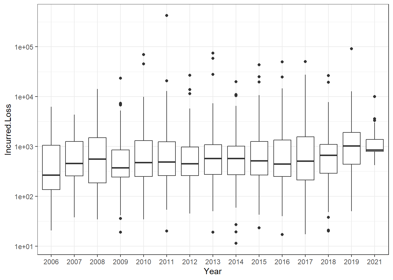
c. Loss Distributions over Time. There are 1835 incurred losses in the dataset with all available years (yet omitting claims less than 10). Figure 1.3 shows that the distribution of incurred losses is stable over the period 2015-2019, inclusive. Produce a comparable figure for the entire period.
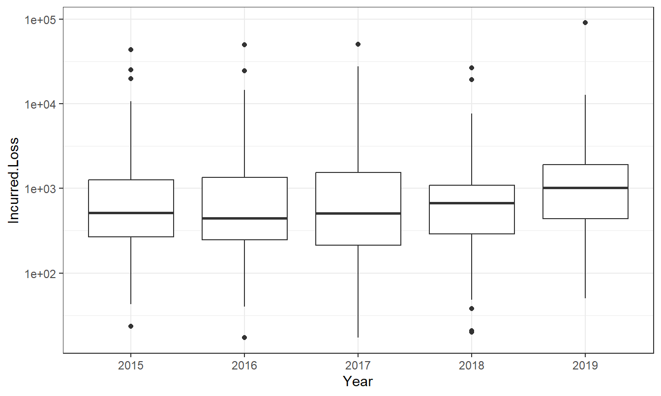
Figure 1.3: Distribution of Travel Losses by Year
d. Summary Statistics. In addition to graphs, it can be helpful to display several summary statistics. For the five year period 2015-2019, produce a set of summary statistics.
Solutions for the Travel Claims Exercise
Exercise 1.2. Group Personal Accident. Group personal accident insurance offers financial protection in case of injury or death resulting from an incident that occurs on the job. Group personal accident offers insurance coverage and liability insurance protection against accidental death or injury. The insurance covers students and ANU’s voluntary workers; ANU workers are covered through another system known as “workers’ compensation.”
Several limits apply including 1,000,000 for the period of insurance, 600,000 for non-scheduled flights, and others. These limits were not reached in the data we consider. For this coverage, there is a “7 day excess” for weekly benefits but none for general benefits. The database documentation provided to us, and the data we provide, do not indicate whether the excess has been triggered; we have only paid claims. Because of the relatively small size of this class of insurance, we ignore the effects of deductibles for this line.
The data provided to us are maintained by the insurer, Chubb. These data began in underwriting year 2007 and were accessed on 29 July 2022. You can retrieve the data by going to Appendix Section 22.3.
a. Claim Frequency. From this data set, there are 148 incurred claims. Of these claims, there are 35 zeros and an additional 0 claims where the incurred claim is less than 10. We omit these claims in our analysis. Table 1.11 shows the count of claims for years 2015-2019, inclusive. Produce a comparable table of claims frequency for the entire period, omitting claims that are less than 10.
| 2015 | 2016 | 2017 | 2018 | 2019 |
|---|---|---|---|---|
| 4 | 7 | 16 | 11 | 9 |
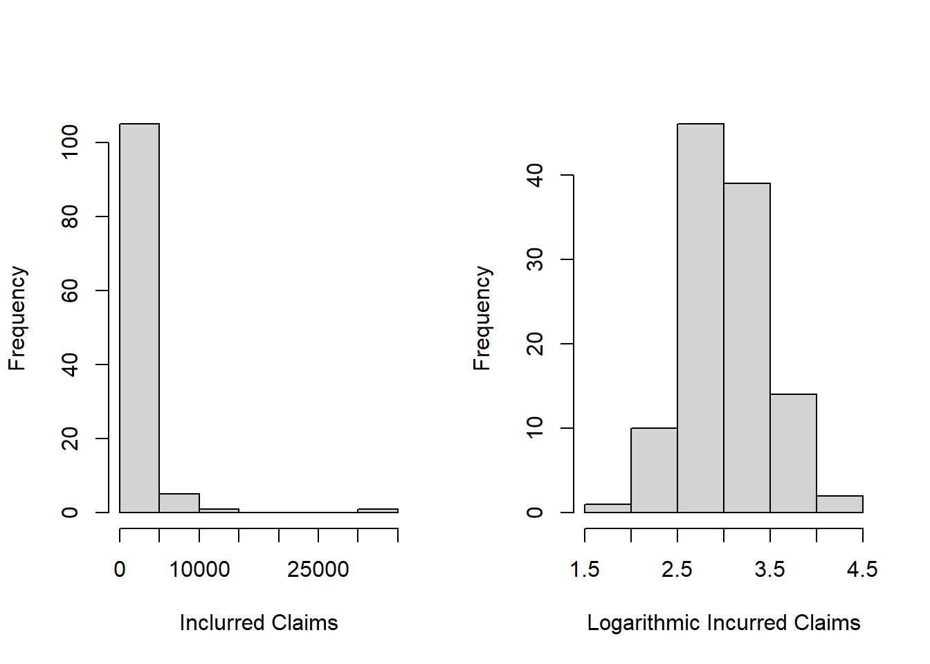
b. Skewness of Claims Severity Distribution. The left-hand panel of Figure 1.4 shows a histogram of incurred claims that reveals the right-skewed nature of this distribution. The right-hand panel shows the same claims but on the log (base 10) scale; this plot demonstrates that the log transform can symmetrize a distribution. These plots are for the 2015-2019 data. Replicate this work, using incurred claims for all available years (still omitting those less than 10).
c. Summary Statistics. Produce summary statistics for both claims and log claims using all available years (still omitting those less than 10). Comment on the relationship between the mean and the median for both claims and log claims, relating this to the symmetry of the distributions observed in part (b).
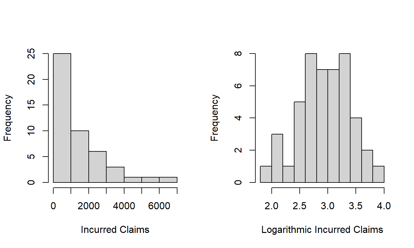
Figure 1.4: Distribution of Incurred Claims 2015-2019
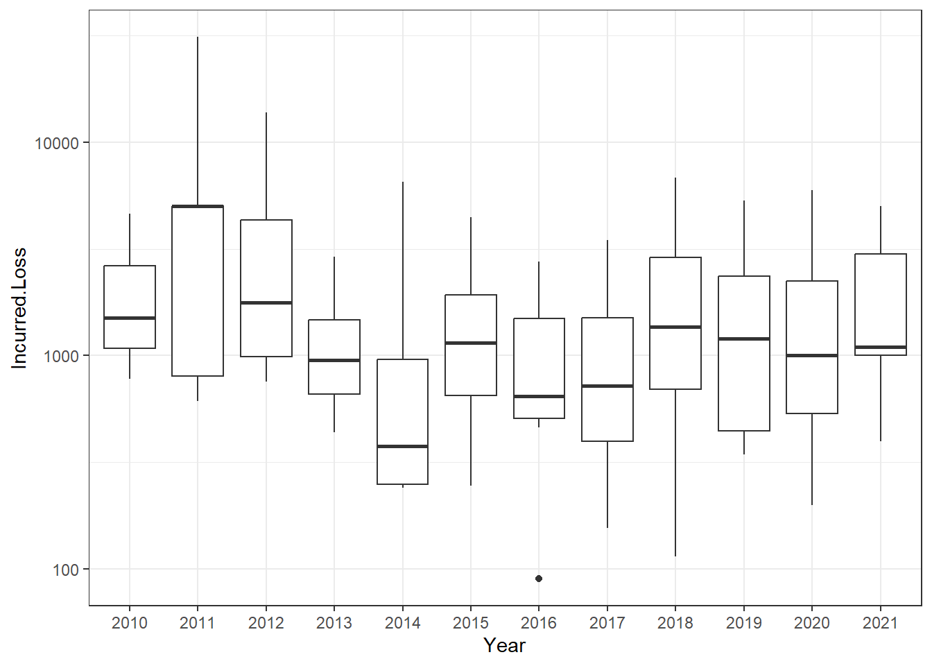
d. Loss Distributions over Time. There are 112 incurred losses. Figure 1.5 indicates that the incurred losses are stable over the period 2015-2019, inclusive. Produce a comparable figure for the entire period and comment on the stability of the distribution.
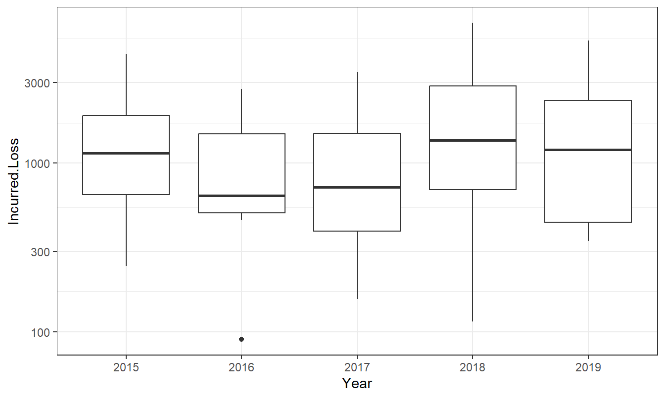
Figure 1.5: Distribution of Group Personal Accident Losses by Year
Solutions for the GPA Claims Exercise
Exercise 1.3. Motor Vehicle. This policy covers ANU’s vehicles including cars, vans, utilities, and motorcycles. There are two parts to this coverage, one for comprehensive damage to the insured vehicles and a second for legal liability. The comprehensive coverage for loss or damage is essentially limited by the market value of the insured vehicle. For legal liability, there is a $50 Million upper limit for all claims arising from the one accident or series of accidents resulting from the one original cause. There is also another upper limit (that is lower than 50 million) when the vehicle is used for transportation of dangerous goods.
The data available contain the amount paid by the insurer (Vero Insurance Limited) which is the focus of our initial analysis. In addition, the data also contains a deductible (called an “excess” in the data file) that we explore in later parts.
The data provided to us are maintained by the insurer, Vero Insurance Limited. These data began in underwriting year 2012 and were accessed on 8 August 2022. You can retrieve the data by going to Appendix Section 22.4.
a. Adjust for Zeros. From this data set, check that:
- there are 318 incurred claims.
- Of these claims, there are 50 zeros and
- an additional 0 claims where the incurred claim is less than 10.
Remove these claims in your analysis, so that there are 268 incurred claims.
b. Claim Frequency. Produce a table that shows the count of claims for the entire period.
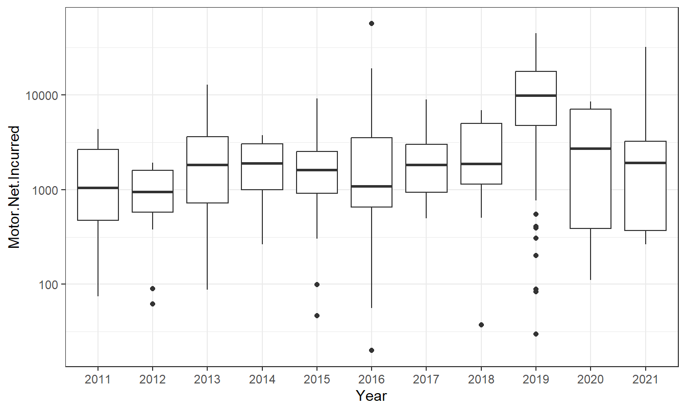
c. Loss Distributions over Time. Produce a figure that shows the distribution of motor vehicle paid amounts over time and comment on the stability of the distribution.
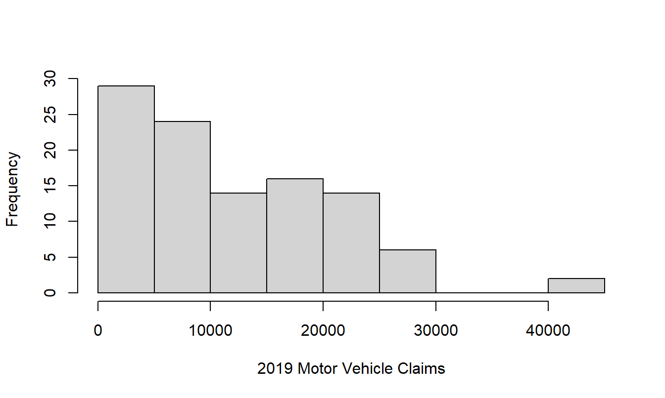
d. Year 2019. In your analysis from the prior steps, you may have noticed the unusual aspects of year 2019. In that year, ANU suffered extensive damage from a hailstorm that increased the frequency of claims as well as the severity. Produce a histogram of paid claims for that year.
e. Deductibles. For each event, or series of events arising from the one originating cause, ANU bears the amount of the excess in respect of each and every insured vehicle, unless stated otherwise. The standard deductible (or excess) in the dataset is 1000. However, a cursory examination of the dataset shows tremendous variation by vehicle and over time. Replicate Table 1.13 that shows, for each year, the number of claims with zero excess, positive excess less than 1000, an excess equal to 1000, and an excess greater than 1000.
| UW.Year | Num 0 | Num 0-1000 | Num = 1000 | Num >1000 | Total |
|---|---|---|---|---|---|
| 2011 | 1 | 1 | 7 | 0 | 9 |
| 2012 | 1 | 2 | 13 | 0 | 16 |
| 2013 | 4 | 1 | 22 | 0 | 27 |
| 2014 | 0 | 0 | 11 | 0 | 11 |
| 2015 | 1 | 1 | 14 | 0 | 16 |
| 2016 | 6 | 1 | 19 | 0 | 26 |
| 2017 | 16 | 0 | 4 | 1 | 21 |
| 2018 | 19 | 0 | 1 | 0 | 20 |
| 2019 | 99 | 0 | 6 | 0 | 105 |
| 2020 | 5 | 0 | 0 | 0 | 5 |
| 2021 | 10 | 0 | 0 | 0 | 10 |
(Deductibles. We recommend that motivated readers extend our analysis to account for this deductible in both the severity and frequency.)
Solutions for the Motor Vehicle Claims Exercise
1.5 Further Resources and Contributors
If you would like additional practice with R coding, please visit our companion LDA Short Course. In particular, see the Introduction to Loss Data Analytics Chapter.
Contributor
- Edward (Jed) Frees, University of Wisconsin-Madison and Australian National University, is the principal author of the initial version and second edition of this chapter. Email: jfrees@bus.wisc.edu for chapter comments and suggested improvements.
- Chapter reviewers include: Yair Babad, Chunsheng Ban, Aaron Bruhn, Gordon Enderle, Hirokazu (Iwahiro) Iwasawa, Dalia Khalil, Bell Ouelega, Michelle Xia.
This book introduces loss data analytic tools that are most relevant to actuaries and other financial risk analysts. We have also introduced you to many new insurance terms; more terms can be found at the NAIC Glossary (2018).

This work is licensed under a Creative Commons Attribution 4.0 International License.
