Chapter 4 Contingent Payment Techniques

\(\require{enclose}\)

Chapter Preview. We have now learned the foundations of life contingencies through Chapter 2 survival modeling and Chapter 3 discounting of contingent cash flows. This chapter provide extensions and variations to exhibit the richness of applications.

Specifically, Section 4.1 presents a relatively minor extension theoretically, allowing for \(m^{th}\)ly cash flows, that has extensive practical ramifications for retirement benefits, other life contingent annuities, and premium payment plans. Section 4.2 sharpens our intuition about survival modeling by linking the choice of a survival dataset to an application under consideration; when the link is not appropriate, important biases can arise. Section 4.3 provides economic motivation for some of the measures summarizing insurance features introduced in Chapter 3; this motivation provides insights as why some of these are so important in practice. Through a variety of examples, Section 4.4 emphasizes that the framework for life contingent benefits applies to contingent payment problems that go beyond applications restricted to the life insurance industry.

4.1 Contingent Cash Flows Occurring \(m^{th}\)ly

---

In this section, you learn how to:

• Discount random cash flows where cash flows occur more frequently than once a year.
• Compute actuarial present values when mortality is available on a continuous basis.
• Compute actuarial present values when mortality is available annually using a uniform distribution of deaths assumption.

---

This section extends Chapter 3 by considering cases where cash flows occur more frequently than once a year. For example, it is common for retirement benefits to be paid on a monthly basis while a person is alive. As another example, premiums might be paid twice a year, as long as the policyholder is alive and the contract is in force. We use \(m\) to denote the number of payments per year. For the retirement benefits example, we would use \(m=12\) and for premiums, \(m=2\). Other common examples are \(m=4\) for quarterly cash flows, \(m=52\) for weekly, and so forth. We will even consider the case where the number of payments becomes arbitrarily large, \(m \to \infty\), corresponding to a cash flow at the moment an event such as death occurs.

When describing benefits paid discretely, we started in Chapter 3 with annual payments because mortality tables have traditionally been presented on an integer age basis. In addition, business requirements such as insurance company financial reporting is done routinely on an annual basis. Nonetheless, as described above, there are also important situations where payments occur other than annually (typically more frequently, although payments once every, e.g., two years are certainly plausible).

4.1.1 Basic Concepts

To appreciate the concerns when transiting from an annual to an \(m^{th}\)ly basis, here is a modified version of Figure 3.1.

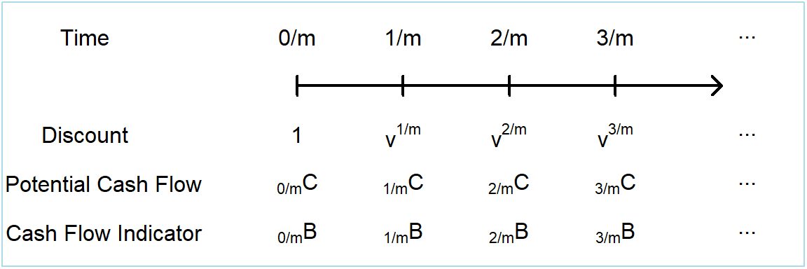
Figure 4.1: Timeline of \(m^{th}\)ly cash flows with uncertainty

Similar to equation (3.2), the present value \(PV\) random variable can be summarized as

\[ \begin{array}{l} PV = \sum_{r=0}^{\infty} v^{r/m} ~_{r/m}C~_{r/m}B~ ~,\\ \end{array} \tag{4.1} \]

using \(r\) is a counter for the number of \(m^{th}\)ly units. For probabilities associated with the cash flow indicator, as we saw in Chapter 3, we are concerned with payments either at the death or the survival of a policyholder age \(x\). That is,

\[ \mathrm{E} \left(_{r/m}B\right) = \left\{ \begin{array}{cccc} \Pr\left(\frac{r-1}{m} < T_x \le \frac{r}{m}\right) & = & ~_{(r-1)/m} p_x - ~_{r/m} p_x& {\small \text{ prob of death}} \\ \Pr\left(T_x \ge \frac{r}{m}\right) & =& ~_{r/m} p_x & {\small \text{ prob of survival} }.\\ \end{array} \right. \tag{4.2} \] As many readers will recall from their study of interest theory, if we think of a discount factor \(v^t = (1 + ~_t i)^{-t}\) in terms of a spot rate of interest \(~_t i\), then there is no difficulty at all in discounting at non-integer times. In addition, suppose that the survival model can be expressed in terms of continuous time, such as the analytic laws of mortality in Section 2.3 or their extended versions in Section 2.6. In these cases, thinking of the unit of time as a year is a mere convenience and no additional theoretical extensions are required for handling \(m^{th}\)ly cash flows.

Uniform Distribution of Deaths. Only in the case where we have annual mortality with \(m^{th}\)ly cash flows are some extensions required. And we already started on this in Section 2.4.4 where fractional year assumptions were introduced. To see how this works with \(m^{th}\)ly cash flows, we use the uniform distribution of death (UDD) assumption so that we can express \(~_t p_x = 1 - t \times q_x\), for \(0 \le t \le 1\). Thus, using \(j\) is a counter for the number of \(m^{th}\)ly units within a year, we have

\[ ~_{j/m} p_x = 1- \frac{j}{m} \times q_x, \ \ \text{for } j= 0, 1, \ldots, m-1. \] For integer \(k=0, 1, \dots\)

\[ ~_{k+j/m} p_x = ~_k p_x \times ~_{j/m} p_{x+k}= ~_k p_x \times \left(1- \frac{j}{m} \times q_{x+k}\right). \] Here, to calculate the probability of a life aged \(x\) surviving \(k+j/m\) years, we first calculated the probability of surviving \(k\) (integer) years and then, conditional on having attained age \(x+k\), applied the UDD assumption to calculate the probability of surviving an additional \(j/m\) fraction of a year. These expressions, together with equations (4.1) and (4.2), are enough to compute an expected present value for an \(m^{th}\)ly version of any of the Chapter 3 cash flows.

4.1.2 Illustrative Cash Flows

Let us see how these ideas work with a few illustrative examples. To begin, we start by assuming that we have a continuous time probability model and so no simplifying assumptions are needed.

Example 4.1.1. Whole Life Insurance with \(m^{th}\)ly Payments with Continuous Time Mortality. For this contract, the benefit is paid at the end of the \(m^{th}\)ly period in which death occurs. Let us return to the familiar Example 3.2 that used the Section 2.6 mortality. We consider the baseline case in Example 3.2 that you will recall is a healthy female who is not a smoker, not obese, and has an average blood pressure level equal to 114. The interest rate is a constant 4%.

To calculate the expected value of this policy, we may use equations (4.1) and (4.2) directly with the potential cash flows identically equal to one \(~_{k/m}C \equiv 1\). The resulting expected present value is

\[ \begin{array}{rl} A_{{\bf{x}}}^{(m)} &= \sum_{r=0}^{\infty} ~v^{(r+1)/m} \{ ~_{r/m} p_x - ~_{(r+1)/m} p_x \} ,\\ \end{array} \]

an expression that introduces the common actuarial notation for the expected present value of this contract. The superscript \(~^{(m)}\) denotes \(m^{th}\)ly cash flows. Figure 4.2 summarizes the expected presented values by age \(x\) over choices of \(m=1,2,4, 12\). As is evident from the plot, these values are close and in fact ordered as

\[ A_x = A_x^{(1)} \le A_x^{(2)} \le A_x^{(4)} \le A_x^{(12)} ~. \]

The annual expected presented value, \(A_x = A_x^{(1)}\), is the smallest because it is the contract with payments potentially farthest in the future. For example, if a person dies just before one month into a contract year, then the payment is 11 months after death. In contrast, it is five months after death when \(m=2\), two months later for \(m=4\) and virtually instantaneous for \(m=12\). So, the very largest the separation that could be in Figure 4.2 is \(1/(1+i) = 1/1.04 \approx 0.96\), suggesting that these expected present values will be close to one another.

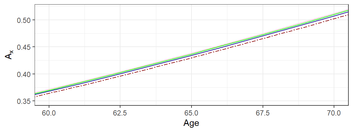
Figure 4.2: Life Insurance by \(m^{th}\)ly Payments. The dark red dashed represents expected present values based on annual cash flows with \(m=1\). The other lines are for \(m=2, 4, 12\), increasing in that order.

Example 4.1.2. Whole Life Insurance with \(m^{th}\)ly Payments with Annual Mortality. Continuing Example 4.1.1, we no longer assume that a continuous time mortality model is available but we have only traditional life table mortality at integer (or annual) ages.

To calculate the expected value of the policy, we follow the procedure of splitting up the payment stream into yearly intervals and then applying the UDD assumption within each year. The details follow.

\[ \begin{array}{rl} A_{{\bf{x}}}^{(m)} &= \sum_{r=0}^{\infty} ~v^{(r+1)/m} \{ ~_{r/m} p_x - ~_{(r+1)/m} p_x \} \\ &= \ \sum_{k=0}^{\infty} \sum_{j=0}^{m-1} v^{k+(j+1)/m} \{ ~_{k+j/m} p_x - ~_{k+(j+1)/m} p_x \} \\ &=_{UDD} \sum_{k=0}^{\infty} ~_k p_x \left\{\sum_{j=0}^{m-1} v^{k+(j+1)/m} \left( \frac{1}{m} \times q_{x+k}\right) \right\} \\ &= \sum_{k=0}^{\infty} ~_k p_x ~q_{x+k} \left\{\frac{1}{m} \sum_{j=0}^{m-1} v^{k+(j+1)/m} \right\} ~.\\ \end{array} \]

To simplify the presentation, we further assume a constant spot rate \(i\) so that \(v^t =(1+i)^{-t}\). With this, we can employ standard geometric sums that many readers will recall from interest theory,

\[ \frac{1+i}{m} v^{1/m}\sum_{j=0}^{m-1} v^{j/m} = \frac{1+i}{m}v^{1/m}\frac{1-v}{1-v^{1/m}} = \frac{i}{i^{(m)}} ~, \\ \]

where \(i^{(m)} = m\left[(1+i)^{1/m}-1\right]\) is the actuarial symbol for a \(m^{th}\)ly interest rate. This yields

\[ A_{{\bf{x}}}^{(m)} = \frac{i}{i^{(m)}} A_x ~. \]

This equation exhibits a constant relationship between the annual expected value of a whole life insurance and one on an \(m^{th}\)ly basis. Also from interest theory, a simple (Taylor series) approximation shows that \(\frac{i}{i^{(m)}} \approx 1 + \frac{i}{2}(1-\frac{1}{m})\), indicating the proximity between these expected present values.

Example 4.1.3. Term Life Annuity with \(m^{th}\)ly Payments. For a more complex example, we now consider the case of an \(n\) year term life annuity with \(m^{th}\)ly payments in advance. By convention, when presenting actuarial annuity symbols, each payment (when the person is alive) is assumed to be \(~_{r/m}C \equiv 1/m\), not 1. This is so that we can readily compare annuities with different payment plans, for example, quarterly to monthly payments, because they both pay a sum of 1 over the year if the annuitant survives.

Based on equation (4.1), and similar to equation (3.15), the random present value of payments is \(PV = \frac{1}{m} \sum_{r=0}^{nm-1} v^{r/m} ~I(T_{\bf{x}} \ge r/m)\). With this and equation (4.2), the expected present value is

\[ \begin{array}{rl} \ddot{a}_{{\bf{x}}:\enclose{actuarial}{n}}^{(m)} &= \frac{1}{m} \sum_{k=0}^{n-1} \left\{\sum_{j=0}^{m-1} v^{k+j/m} ~_{k+j/m}p_{\bf{x}}\right\} \\ &=_{UDD} \frac{1}{m} \sum_{k=0}^{n-1} ~_k p_x \left\{\sum_{j=0}^{m-1} v^{k+j/m} \left(1- \frac{j}{m} \times q_{x+k}\right) \right\} ~.\\ \end{array} \]

To simplify the presentation, we again assume a constant spot rate \(i\) so that \(v^t =(1+i)^{-t}\). After some pleasant algebra, one can show that

\[ \begin{array}{rl} \ddot{a}_{{\bf{x}}:\enclose{actuarial}{n}}^{(m)} &=_{UDD} \frac{d}{d^{(m)}} \ddot{a}_{{\bf{x}}:\enclose{actuarial}{n}} - v ~\beta(m) A_{{\bf{x}}:\enclose{actuarial}{n}} ^ {1} ~,\\ \end{array} \] where \(d^{(m)} = m\left[1- v^{1/m}\right]\) is an \(m^{th}\)ly discount factor and \(\beta(m) = \frac{i-i^{(m)}}{i^{(m)}d^{(m)}}\) is another factor based only on the interest rate, not the survival model. You can check, either using Taylor series approximations or by calculating using several values of \(m\) and \(i\), that \(\beta(m) \approx \frac{m-1}{2m}\), an approximation that is very useful for interpreting this expected present value.

Verify Development of EPV for Term Life Annuity with mthly Payments

First recall some standard notation from interest theory:

\[ \begin{array}{cccccc} i^{(m)} = m\left[(1+i)^{1/m}-1\right] & & d^{(m)} = m\left[1- v^{1/m}\right] \\ \alpha(m) = \frac{i}{i^{(m)}}\frac{d}{d^{(m)}} & & \beta(m) = \frac{i-i^{(m)}}{i^{(m)}d^{(m)}} \\ \end{array} \]

Next, from standard geometric sums employed in interest theory, we have

\[ \begin{array}{cccccc} \frac{1}{m}\sum_{j=0}^{m-1} v^{j/m} &=& \frac{1}{m}\frac{1-v}{1-v^{1/m}} & = \frac{d}{d^{(m)}} \\ \end{array} \]

and \[ \begin{array}{cccccc} \frac{1}{m}\sum_{j=0}^{m-1} j~v^{j/m} &=& \frac{v^{1/m}}{m} \frac{1-v}{(1-v^{1/m})^2} - \frac{v}{1-v^{1/m}} \\ &=& \frac{v^{1/m}}{(1-v^{1/m})} \frac{d}{d^{(m)}} - \frac{mv}{d^{(m)}} \\ &=& \frac{m}{i^{(m)}} \frac{d}{d^{(m)}} - \frac{mv}{d^{(m)}} \\ &=& mv \left( \frac{i}{i^{(m)}d^{(m)}} - \frac{1}{d^{(m)}} \right) \\ &=& mv ~\beta(m) \\ \end{array} \]

This yields

\[ \begin{array}{rl} \ddot{a}_{{\bf{x}}:\enclose{actuarial}{n}}^{(m)} &=_{UDD} \frac{d}{d^{(m)}} \sum_{k=0}^{n-1} v^{k} ~_k p_x - mv ~\beta(m) \frac{1}{m} \sum_{k=0}^{n-1} ~_k p_x q_{x+k} \\ &= \frac{d}{d^{(m)}} \ddot{a}_{{\bf{x}}:\enclose{actuarial}{n}} - v ~\beta(m) A_{{\bf{x}}:\enclose{actuarial}{n}} ^ {1} \\ &\approx \ddot{a}_{{\bf{x}}:\enclose{actuarial}{n}} - \frac{m-1}{2m} . \\ \end{array} \]

4.1.3 Contingent Cash Flows in Continuous Time

By cash flows in “continuous time,” we are thinking of a situation where \(m\) becomes arbitrarily large. So, we could start with monthly (\(m=12\)), go to weekly (\(m=52\)), proceed to daily (\(m=365\)), and so forth. As we will see, there is little difference between a contract with daily payments versus instantaneous payments. However, the model with instantaneous payments (\(m=\infty\)) is actually easier because we do not have to distinguish between payments at the beginning versus the end of the period.

Models with instantaneous payments are easier to interpret and analyze in life insurance in contrast to life annuities. Because insurers typically pay benefits quickly upon the death of a policyholder, a model with payments at the moment of death is a better approximation than one that pays at the end of the year (\(m=1\)). Theoretically, one can think of a continuous life annuity as an approximation to a life annuity that pays 1/365 on a daily basis. However, given that life annuities are predominantly employed on a monthly (\(m=12\)) and quarterly (\(m=4\)) basis, we focus our attention on life insurance products in continuous time.

It is possible to express present value random variables using a limit of equation (4.1) but it is much cleaner to simply utilize the moment of death random variable \(T_x\) with basic contract definitions, as follows:

\[ PV = \left\{ \begin{array}{cc} v^{T_{\bf x}} & {\text{whole life}} \\ v^{T_{\bf x}}I(T_{\bf x} \le n) & {n\text{ year term}} \\ v^n I(T_{\bf x} >n) & {n\text{ year pure endowment}} \\ v^{T_{\bf x}}I(T_{\bf x} \le n) +v^n I(T_{\bf x} >n) & {n\text{ year endowment}}.\\ \end{array} \right. \]

Expected present values can be readily determined using first principles. To illustrate, for a whole life insurance that pays at the moment of death, we have

\[ E(PV) = \int_0^{\infty} ~ v^t ~_t p_x \mu_{x+t} dt = \bar{A}_x . \]

For notation, we could use \(~^{(\infty)}\) to signify payments with an infinite number of payment periods. However, it is traditional and part of International Actuarial Notation to use a bar (\(\bar{\cdot}\)) to denote payments at the moment of death. See Appendix Section 9.2 for more on actuarial notation.

Similarly for an \(n\) year endowment, we have

\[ \begin{array}{ll} E(PV) &= \int_0^n ~ v^t ~_t p_x \mu_{x+t} dt + \int_n^{\infty} ~ v^n ~_t p_x \mu_{x+t} dt \\ &= \int_0^n ~ v^t ~_t p_x \mu_{x+t} dt + v^n ~_n p_x \\ & = \bar{A}_{{\bf{x}}:\enclose{actuarial}{n}} . \end{array} \]

When a continuous time probability model is available, then these integrals can be computed directly (although they sometimes require numerical integration software). An alternative approach is to use the approximations based on \(m^{th}\)ly payments introduced in the prior section and let \(m \to \infty\). For example, for the whole life assuming UDD, we have

\[ \bar{A}_x = \lim_{m \to \infty} A_x^{(m)} = \lim_{m \to \infty} \frac{i}{i^{(m)}} A_x = \frac{i}{\delta} A_x , \]

where \(\delta = \ln(1+i) = \lim_{m \to \infty}i^{(m)}\) is the force of interest, from interest theory.

Section Structure Discussions

Structure discussion.

This section is general in the sense that it:

• integrates both life and annuity contracts under one umbrella
• readily allows variable interest rates and continuous time mortality without making assumptions such as UDD

However. It does not relate insurance to annuity coverages. It only does second moments indirectly. It does not provide details for many contracts.

At this stage, not sure how far to push this because I don’t know how important the topic is relative to the other material…

Probably could use lots of exercises.

---

• Introduce classical actuarial PV symbols, variance calculations
• Calculation approaches
  • Start with continuous time hazard survival models
  • Describe approximations based on life table functions
  • Differential equations? Continuous analog to the recursive formulas of insurances/annuities. (Develop this in the problem set).

---

• Use life annuities to motivate why it matters to account for more frequent premium and benefit payments
• Use life insurance to motivate why it a continuous payment model is a useful approximation (e.g., contractually obligated to settle payment immediately, subject to death confirmation)

---

• Review the present value random variable and moments. Draw timeline with more frequent payments.
• Introduce mthly insurances and annuities, as well as their relationship
• Introduce classical actuarial PV symbols, variance calculations
• Why is the frequency important? Demonstrate magnitude of difference in expected present values of payments (e.g., make a table of EPV vs various m) (without showing how calculations are done)

---

• Describe implementation using the continuous time Cox hazard model
• When life table is used, interim timing can be approximated via UDD, exponential. Possible extensions (or in appendices, problem sets):
  • Does UDD work for all ages or covariates? Is there need to empirically investigate using our available data?
  • Should we further explore other approximations using the model T_x = K_x +R_x, where R_x is the fractional term?
  • Approximations of life annuities based on Woolhouse. Derivation is via Taylor’s expansion. (might also be an exercise)

4.2 Sampling Bias

---

In this section, you learn how to:

• Describe different subpopulations that are commonly used in actuarial practice, including variations by country and by areas of practice (insured lives, annuitant, and general population).
• Interpret how using different subpoplulations may result in a sampling bias.
• Quantify the impact of sampling bias on actuarial present values.

---

In Chapter 2 we saw that survival distributions, expressed as mortality rates, can vary not only by age and sex but also by other attributes such as smoking status, systolic blood pressure, and so forth. This naturally raises the question as whether these attributes are important in actuarial practice. To frame this question, this section reviews the statistical concept of sampling bias in the context of actuarial applications.

4.2.1 Population Subsets and Sampling Bias

To illustrate differences among different samples, or subsets of a population, we consider three samples commonly used in actuarial practice:

• insured lives, individuals who have purchased life insurance,
• annuitant or pensioner lives, individuals who have either purchased an annuity or are a pensioner and so enjoy an annuity by participating in a retirement system, and a
• general population, where there is no requirement for insurance/annuity participation.

To compare these three samples, we examine a specific case.

Example 4.2.1. Korean Mortality by Insured Status. Here, we consider female mortality from South Korea for year 2007. The insured lives and annuitant rates were drawn from a database organized by the Society of Actuaries, https://mort.soa.org/. The general population data are drawn from the Human Mortality Database. These data are organized in Appendix Section 8.5.

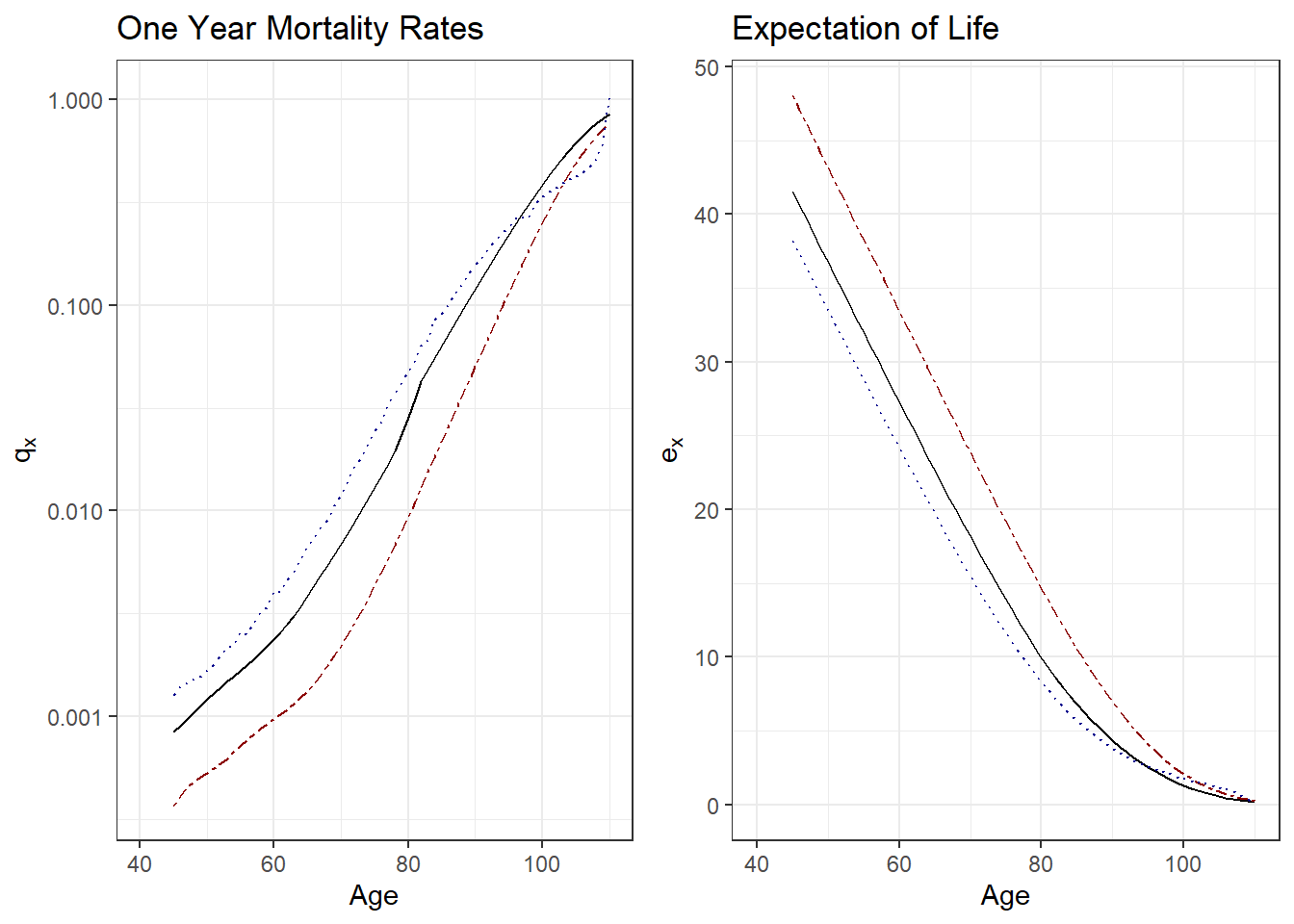
Figure 4.3: Mortality by Insured Status. The left-hand panel summarizes mortality by one year rates \(q_x\) by age \(x\), the right-hand panel shows it by expectation of life \(e_x\). Both panels show three sampling frames: the solid black line is for insured lives, the dark-red dashed lines is for pension (annuitant) lives, and the dotted blue line represents the general population.

Figure 4.3 compares these three samples using one year mortality rates \(q_x\) and expectation of life \(e_x\). Except for the highest ages where data are less reliable, the left-hand panel shows that pensioner (annuitant) mortality is the lowest among the three, followed by insured lives, and then the general population. The right-hand panel shows the same pattern, with pensioners enjoying the longest life expectancy and the general population showing the lowest.

These patterns are commonly observed in actuarial practice. Individuals electing to purchase an annuity, or choosing an annuity option at retirement, generally consider themselves to be in good health. If they are in poor health, then they would not take on a contract that pays as long as they live. One might also elect to apply that same logic to the purchase of life insurance; that is, reason that only those who are in poor health purchase life insurance. However, insurers typically require individuals applying for life insurance to take a medical examination. So, by this selection mechanism, mortality for insured lives is also better than the general population.

---

In the language of statistics, a sampling error occurs when the sampling frame, the list from which the sample is drawn, is not an adequate approximation of the population of interest. A sample must be a representative subset of a population, or universe, of interest. An example of a representative subset is a sample drawn at random. With substantial sample errors, the summary measure of the sample, the statistic, is not an adequate approximation of the corresponding summary measure of the population, the difference defined as a bias. If the sample is not representative, taking a larger sample does not eliminate bias, as the same mistake is repeated over again and again.

So, using data from a sample that is not representative of a population of interest can result in sampling bias. For example, an analyst investigating an insurance product might use (typically convenient) population mortality instead of a more appropriate insured lives mortality; this mismatch results in sampling bias. As an another example, one might use insured lives mortality in lieu of pensioner mortality when valuing a retirement option for an insurance product. It is also common to use experience from one country to approximate outcomes in another. To illustrate, the following example compares experience among Poland, Japan, and the United States.

Example 4.2.2. Mortality by Country (Japan, Poland, and the United States). This example focuses on population mortality and so recent 2019 experience is available from the Human Mortality Database. These data are organized in Appendix Section 8.6. In addition to classification by country, we also look at experience by sex and age as these distinctions are well known.

Figure 4.4 compares one year mortality rates among the three countries; the left-hand panel is for female experience and the right-hand is for males. Both panels demonstrate that Japan has the lowest mortality rates. The relationship between the United States and Poland is more complicated. For females, experience is roughly the same for ages above 50 although Poland has lower mortality rates for younger females. Younger polish men also have lower mortality rates than men in the US but the reverse is true for those older (than approximately 45).

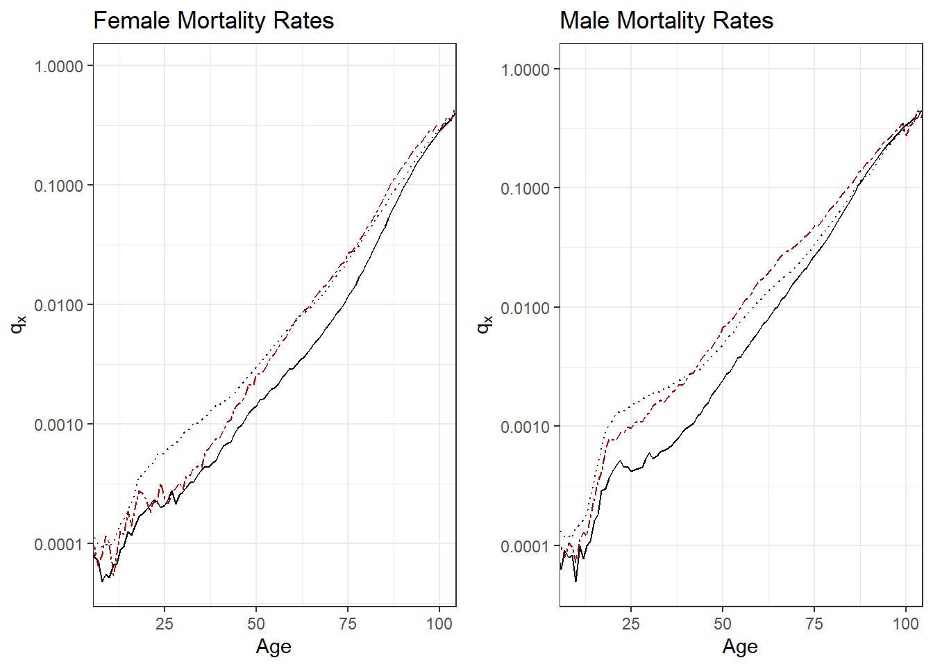
Figure 4.4: 2019 Mortality Rates by Country. Both panels show three countries that represent different sampling frames: the solid black line is for Japan, the dark-red dashed line is for Poland, and the dark-blue dotted line represents the United States. The left-hand panel summarizes female mortality, the right-hand panel represents males.

---

Although we did not explicitly mention the sample sizes in Examples 4.2.1 and 4.2.2, they are large, and so do not confuse the issue of sampling bias with the uncertainty that arises from small data sets. The relationships observed among annuitants, insured lives, and general population as well as among countries demonstrated in these examples are commonly observed. To substantiate this claim, mortality rates from around the world are readily available at https://mort.soa.org/ and Human Mortality Database. Readers are encouraged to visit these primary sources and follow up with their own analyses.

4.2.2 Sampling Bias in Actuarial Practice

In the prior subsection, we defined the concept of sampling bias and established that it could be a real concern in commonly encountered applications. However, you might have noticed that the vertical axes in the one year mortality rate graphs in Examples 4.2.1 and 4.2.2 are on a logarithmic scale. So the discrepancies among sampling bases seem real but how important are they in actuarial applications?

To get insights into this question, we can use the different mortality distributions and, with the tools we learned in Chapter 3, express them in terms of expected present values.

Example 4.2.1. Mortality by Insured Status - Continued. We use the female South Korean mortality experience introduced in Example 4.2.1 and, for illustration purposes, assume \(i=4\)%. For many new products or regions in the world with less detailed mortality data, it is common to use population mortality data in lieu of more appropriate insured lives or annuitant data. So, using population data, we first compute expected present values for a whole life insurance (\(A_x^{pop}\)) and for a life annuity due (\(\ddot{a}_x^{pop}\)). Next, with the insured lives data, we compute the expected present values for a whole life insurance (\(A_x^{ins}\)). Lastly, with the annuitant lives data, we compute the expected present values for a life annuity due (\(\ddot{a}_x^{ann}\)).

Figure 4.5 summarizes the discrepancies by reporting the ratios. The left-hand panel shows the ratio \(A_x^{ins}/A_x^{pop}\). Except for the very high ages, we see that the ratio is considerably less than one. This is consistent with our earlier observations that population mortality is higher than insured lives mortality. If we think of the expected present values as representing prices (as developed in the next section), then the ratio also provides a basis for the analyst to decide whether the difference is important. Many insurance markets are competitive and one calculation basis being 90% of the other represents an important financial difference.

The right-hand panel is the ratio \(\ddot{a}_x^{ann}/\ddot{a}_x^{pop}\). Here, the value of annuity under annuitant lives mortality is higher than that under general population mortality. This is consistent with our earlier observations that population mortality is higher than annuitant lives mortality. As with the insurance ratio, for many marketplaces this difference is financially meaningful.

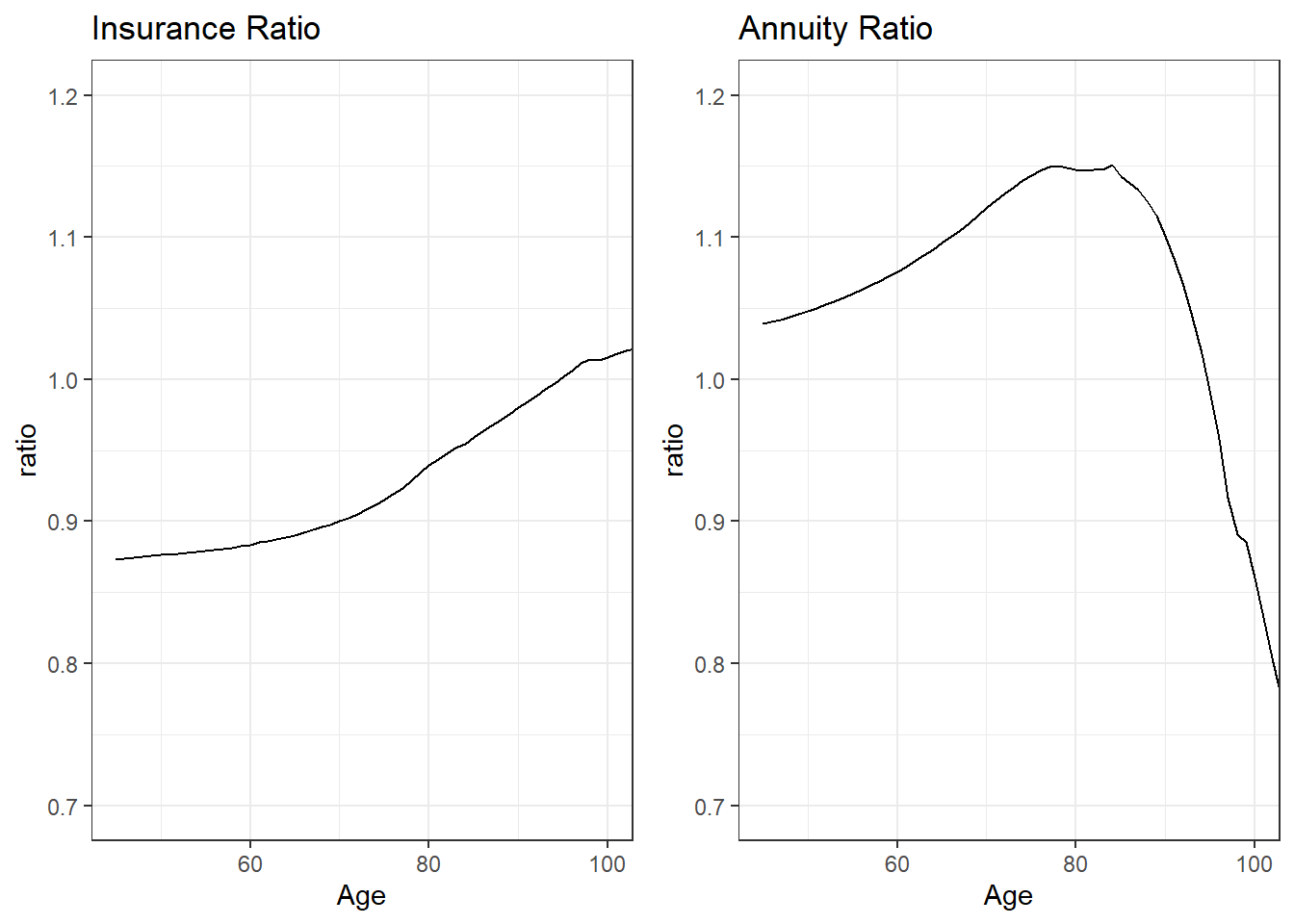
Figure 4.5: Dependence of Expected Present Values on Insured Status. The left-hand panel provides a ratio of \(A_x\) computed using insured lives mortality to that computed using general population mortality. The right-hand panel provides a ratio of \(\ddot{a}_x\) computed using annuitant lives mortality to that computed using general population mortality.

---

An annuity product pays benefits while an individual is alive whereas an insurance product pays benefits upon the death of an insured. So, to a certain extent, these two products offset one another. In financial terms, you can think about an annuity (based on an individual’s survival) as a hedge for insurance (based on an individual’s mortality). In the following Chapter 5 on premiums, we will take advantage of relationships of the form:

\[ A_x + d \ddot{a}_x = 1. \tag{4.3} \]

This is an exact relationship between the expected present values. However, this relationship holds under the assumption that the insurance and annuity expected present values use the same mortality. To dispel the notion that this holds more generally, Figure 4.6 shows the sum \(A_x^{ins} + d \ddot{a}_x^{ann}\), computed using the mortality and interest assumptions in Example 4.2.1.

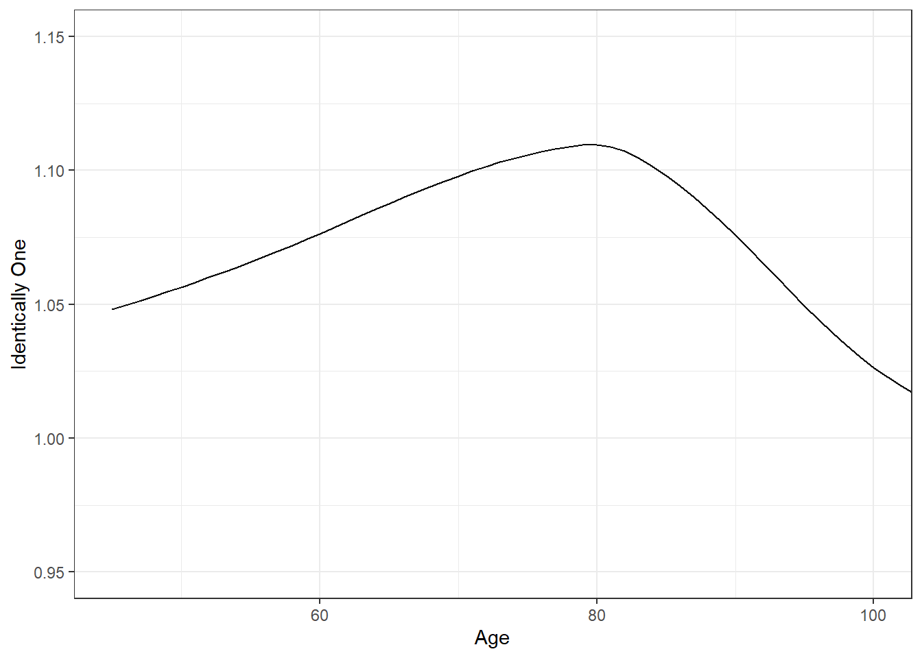
Figure 4.6: The Sum \(A_x^{ins} + d \ddot{a}_x^{ann}\). This sum is plotted versus age \(x\) and is clearly not identical to one, as suggested by equation (4.3).

Exercise Quantify the use of annuity mortality applied to life insurance, and vice-versa, as examples.

---

We motivated this section by questioning whether attributes such as smoking status and systolic blood pressure are important in actuarial practice. In the exercises, readers have the opportunity to determine expected present values of life contingent benefits that vary by these attributes. In this section, we learned we can attribute these discrepancies to differences among population subsets. In the next section, we frame the question of importance in terms of economic interpretations of the expected present values.

Exercises Quantify expected present values of life contingent benefits that vary by smoking status and systolic blood pressure.

4.3 Using Economics to Motivate Insurance Features

---

In this section, you learn how to:

• Interpret the expectation of a random present value as an actuarial present value.
• Define adverse selection and explain how select and ultimate mortality tables provide protection against adverse selection.
• Describe moral hazard with examples from life insurance and explain how it relates to information asymmetry.

---

4.3.1 Actuarially Fair Prices and Risk Classification

You may have noticed in Chapter 3 that we paid special attention to the expected present values associated with random life contingent benefits and even gave them special symbols such as \(A_x\) and \(\ddot{a}_x\). This is because insurance prices are based on these expectation of losses, a concept known as an actuarially fair price.

In a simple model, an actuarially fair price is the result of an assumption of zero profits. Specifically, imagine a homogeneous population where all potential insureds have the same distribution of losses.

• If an insurer charges the expected loss to each insured, then the average profit over many such contracts would be zero by the law of large numbers. If there is only one insurer, then the company has a monopoly and so would charge more than this. It would charge the maximum that consumers are willing to pay (known as first degree price discrimination).
• If another company wishes to enter the marketplace, then it would charge something less than that maximum. With this price, it would take business away from the original insurer but still make a long-run profit if the price exceeds the expectation.
• However, competition in the marketplace will lead the original company to undercut, and so on.
• In the end, all profits will be competed away and – because of price competition – the companies will offer products at their expected value.

One can also interpret fairness from a social justice perspective. One can imagine a group of individuals forming a risk class pooling their losses. Through the pooling mechanism, each person is no longer responsible for their individual loss but rather for their share of the pool’s combined loss. From a moral perspective, the responsibility for the loss can now be thought of as not due to the behavior of the faulty individual but rather attributed to the collective; in this sense, pooling socializes responsibility and creates a sense of shared responsibility among a group of people.

This, combined with a certain understanding of equality and justice, creates a type of insurance solidarity. It is not the same type of solidarity that one thinks of in political movements, which embody a conscious identification with the group, emotional bonds, shared values and beliefs, and so forth. It is solidarity that emphasizes mutual responsibility, reciprocity, and a particular shared understanding of fairness. From this understanding of fairness comes the observation that if members of the pool have the same risk distribution when entering the pool, then they should have the same responsibility for the pool losses. As with economic reasoning, the law of large numbers implies that this share is the expectation of losses.

Actuarially fair pricing is a foundation of insurance pricing. Combining a probabilistic viewpoint of an expected value and an interpretation of fairness, oftentimes the expectation of a present value of a random loss is known as an actuarial present value.

Another foundation of insurance pricing is risk classification, defined to be the grouping of insureds into homogeneous classes. As mentioned above, by “homogeneous” we mean that each insured within a group has the same distribution of potential losses. Even within a homogeneous class of insureds, there clearly will be stark differences after observing their mortality. But, before experience is observed, everyone has the same chance (or distribution of outcomes) in a homogeneous class.

Combining these ideas, one can see how insurance prices in competitive marketplaces are based on an actuarial present value for each risk class. Thus, development of distinct risk classes is a critical to fair insurance pricing.

4.3.2 Selection and Adverse Selection

To develop distinct risk classes, insurers can use their underwriting processes to select subsets of a population. For example, as described in Example 4.2.1, when an individual applies for life insurance, it is common for insurers to require a medical examination. Insurers only issue their so-called “standard” policies to individuals who have passed the medical exam. By this mechanism, they are effectively selecting a subset of the population that is healthier than the general population. (Insurers also issue “substandard” policies, at a higher cost, to those with complicated health histories, like diabetes or heart disease, as well as drug, alcohol, or tobacco abuse.)

However, it is known that these selection effects do not continue indefinitely. For example, Table 4.1 shows an excerpt from individual insurance mortality tables for females from Canada. To help read this table, consider a woman who became insured at age \(x=50\) who initially has a mortality rate of 0.00047; one year later (at age 51) she has a mortality rate of 0.00072. This second rate is higher than 0.00053, the mortality rate for a woman who became insured at age \(x=51\). This suggests that the selection effect is becoming less important. Further, from the table we see that selection effects last for 15 years; thereafter, rates are blended into an “ultimate” column. So for example, consider two females currently age 66 where one purchased insurance 16 years ago at age 50 and the other purchased insurance 15 years ago at age 51. Both have the same ultimate rate, \(q_{66} = 0.01209\).

Table 4.1: Select and Ultimate Female Canadian Mortality Rates

Age	Select=0	Select=1	Select=2	Select=3	Select=4	Select=10	Select=14	Ultimate Mortality	Ultimate Age
50	0.00047	0.00072	0.00095	0.00120	0.00150	0.00455	0.00948	0.01096	65
51	0.00053	0.00080	0.00106	0.00135	0.00169	0.00525	0.01056	0.01209	66
52	0.00059	0.00090	0.00119	0.00152	0.00190	0.00615	0.01163	0.01321	67
53	0.00066	0.00101	0.00134	0.00171	0.00214	0.00704	0.01271	0.01433	68
54	0.00074	0.00114	0.00151	0.00193	0.00240	0.00794	0.01379	0.01546	69

• Individual Life Experience Subcommittee, “Construction of CIA9704 Mortality Tables for Canadian Individual Insurance based on data from 1997 to 2004”, Canadian Institute of Actuaries (2010).
• Accessed: October, 2021 from http://www.cia-ica.ca/docs/default-source/2010/210028e.pdf
• Data retrieved from https://mort.soa.org/ (Table 1458)

Why do insurers bother with the cost and other administrative expenses of requiring a medical exam? They do so because they are concerned with a problem known as adverse selection, defined as a situation when consumers know more about their own risk characteristics than insurers. Specifically, without a medical exam, applicants have more knowledge of their medical history and general health status than the insurer. The problem arises because, without a medical exam requirement, it is more likely that people in poor health would apply for life insurance. People in poor health tend to have higher mortality rates that, as we have seen, results in higher actuarial present values for life insurance products.

Abstracting from this a bit, you can think of the insurance pool as being comprised of two groups, those in good health and those in poor health. Providing a single insurance price for both groups violates the fundamental principle of risk classification. As we did in Section 4.3.1, it is easy to construct scenarios based on two insurers, one recognizing health differences and the other not doing so. In the long-run, the latter company becomes priced out of the marketplace. Insurers argue that by knowing about risk factors such as health status, the entire marketplace is better. Indeed, the entire purpose of risk classification is to mitigate the problem of adverse selection.

In this section, we have seen the selection consequences of introducing, or not, a medical exam. As demonstrated in Table 4.1, when a medical exam is introduced, we are essentially fine-tuning our definition of homogeneous classes by including not only factors such as sex and age but also time since a medical exam was taken. By not requiring a medical exam, we introduce heterogeneity into our risk groups and so lose the advantages associated with risk classification. In the following subsection, we introduce other problem situations that result in heterogeneous risk groups.

4.3.3 Asymmetric Information

Adverse selection occurs when the additional information that the insured has is important and not revealed to the insurers, such as a poor health history. Adverse selection is a type of unequal access to information, known as information asymmetry.

Another type of information asymmetry is moral hazard. In moral hazard, the insurance contract itself changes the distribution of risks. To illustrate, by purchasing insurance, insureds have the incentive to take on more risks (thus increasing the probability of a risky event). For example, after purchasing life insurance, the insured may become decide to take up sky-diving, high-speed race car driving, or a life of crime. If the insurer knows about the risky activity in advance, then appropriate adjustments to the price may be made (or the contract simply not issued). The problem arises if the risky activity is taken on after the contract is issued; prices are based on one set of circumstances, losses based on another. Typically this mismatch results in a loss for the insurer. To mitigate this type of problem, insurers may introduce coverage restrictions. For example, life insurance contracts often do not pay benefits for deaths incurred while committing a crime or participating in an illegal activity.

---

This bit on genetic testing may go into an Appendix or sidebar.

Consumers often purchase life insurance to provide benefits for their loved ones in the event of their untimely demise and thus provide a bit of peace of mind. Moreover, there are other, more subtle, ways that the introduction of an insurance contract can change the behavior of consumers, not all in positive ways. One example is genetic testing. Genetic testing involves a type of medical test that examines chromosomes, genes, or proteins. The results of a genetic test can confirm or rule out a suspected genetic condition or help determine a person’s chance of developing or passing on a genetic disorder. There are many different purposes for testing, including medical (such as diagnosing a genetic disease or predicting disease risk) and non-medical (such as confirming parentage or forensic investigation).

Insurers worry about genetic testing information because of information asymmetry concerns. Like the purchase of life insurance, the decision to undergo genetic testing is voluntary. When a potential policyholder has information about his or her health that is not shared with the insurance company, this could lead to anti-selection where poorer risks purchase more insurance and better risks purchase little or no insurance. From an insurer’s viewpoint, one solution would be to allow insurers to require genetic testing, just as they are allowed to evaluate other aspects (e.g., weight, hypertension, and so forth) of a person’s health.

One way that genetic testing differs from, e.g., blood pressure, is through the impact that it has on a person’s willingness to undergo the testing for fear of being denied life insurance. As summarized by Prince (2019), “Empirical evidence shows that fear of genetic discrimination has led individuals across the globe to refuse to participate in genetic research projects or to fail to undergo recommended clinical testing.” In this way, genetic testing also represents a type of moral hazard in the sense that the presence of an insurance contract can change a person’s behavior.

---

Another implication of moral hazard is that people tend to increase their risk unless given incentives not to. Conversely, people may also reduce their risks when given incentives to do so. Indeed, much of modern risk management is predicated on introducing risk mitigation tools to reduce the impact of insured events. A classic example is the nonsmoker discounts in life insurance.

Another type of information asymmetry can occur when an insurer has less information than other competing insurance companies about the risk levels of its customers (cf. Cather 2018). This can result in cream skimming, because the innovative insurer targets the best risks who, like cream in a container of fresh milk, rise, to the top of a pool of policyholders. To illustrate, consider the Section 4.3.2 that we discussed where one insurer has knowledge of an insured’s health status and another does not. The insurer with this knowledge would target risks in good health because these are the ones, other things being equal, would enjoy a lower present value of benefits paid resulting in greater profits for the insurer.

Later, we may wish to gently insert a bit about discrimination/algorithmic bias.

4.4 Contingent Payment Applications

---

In this section, you learn how to interpret life contingent techniques as applicable more broadly to general contingent payment problems.

---

Our work so far has focused on modeling financial implications of survival as the time to event. This is easy to justify; the life insurance industry represents a major piece of the world economy. For example, in 2019, this industry accounted for 2512 trillions of U.S. dollars in developed (OECD) countries, representing more than 3.9 percent of the global economy (OECD (2020)).

Nonetheless, “life contingent” techniques apply more broadly than only human mortality and so in this section we emphasize by referring to them as “contingent” techniques (omitting the life part). As our first example, Section 4.5 describes a relatively small but quickly growing marketplace on pet insurance where time to survival of pets is the event of interest. As a second example, Section 4.6 introduces disability income insurance. In this latter example, we present applications where the time to event is not the time to death but rather the time to recovery from disability.

These examples illustrate that contingent payment techniques can be used to understand financial implications of a time to event and that event need not be human mortality. Another example that we will see later in the book is the time to death of the first of two people.

Section Structure Discussions

Here are a few more examples that could be included in problems or just mentioned in passing….

1. Consider workers’ compensation where a benefit is paid when a worker gets into an accident (at work) and receives benefit payments for many years. The event time is the sooner of recovery or retirement. General insurance actuaries often don’t worry about time value of money but they should.
2. Time to divorce is a good example used in labor economics extensively. Might use the 2014 paper (https://link.springer.com/content/pdf/10.1007/s13524-013-0278-1.pdf) that has a fitted Cox regression model. (Pension valuation would be an actuarial application.) Other labor economic examples include time in and out of employment, time until first child, and many others.
3. Real Estate Valuation. This is an old, old topic. Shaun Wang did something on it that we can check out, https://www.casact.org/sites/default/files/database/forum_14wforum_wang.pdf. A good possibility.
4. Warranty analysis. This is mentioned in Bowers et al, if I recall. We can check it out.
5. Applications addressing long-term social needs such as climate change. How about long-term costs to society for flood insurance/costs? Related to this, how about long-term expenditures for landfills for when determining the cost of a car?

---

Supporting URLs for Pet Insurance

Will remove these later…

• https://www.protectapet.eu/
• https://www.petinsurance.ie/Content/documents/PolicyDoc/1598_PetInsurance_Policy_IRL_Premier_A5_V3_web.pdf
• https://www.simplegermany.com/best-dog-insurances-germany/
• Verteramo Chiu et al. (2021)

4.5 Pet Insurance

---

In this section, you learn how to:

• Describe the pet insurance market.
• Analyze canine (non-human) mortality and assess factors that impact the survival distribution.
• Compute actuarial present values that summarize the lifelong cost of caring for a pet.
• Summarize the history, regulatory environments, and economics principles affecting the pet insurance marketplace.

---

4.5.1 Introduction to Pet Health Insurance

The COVID pandemic that began in 2019 changed life in many ways. Several studies have reported that as many businesses shifted their employees to remote work-from-home schedules, the demand for acquiring or fostering a new pet grew, Hoffman, Thibault, and Hong (2021). Of course, there are costs associated with these new members of a household, some of which can be reasonably predicted and budgeted for (such as food and toys), others which are unexpected (e.g., kennel boarding of a pet when an emergency trip is to be taken by the owner), and still others that could not be remotely foreseen (e.g., the costs of repairing damages your dog did to buildings, living quarters, or other property). Naturally, insurance is one mechanism for paying for costs not anticipated. Pet insurance is a relatively small portion of the insurance marketplace but, even prior to the onslaught of the COVID pandemic, had been growing rapidly, Malloy (2018).

Types of Pet Insurance. As with humans, there are many types of risks associated with pets. If one has a large or aggressive dog, then it may be necessary to purchase third party liability that covers damages your pet may do to other parties (similar to third party auto insurance). Several European countries (e.g., Sweden, Spain, parts of Germany) have requirements that dog owners maintain coverage for liability to third parties for the action of pets. In the U.S., pet owner liability to third parties from injuries caused by common household pets is generally covered by the owner’s homeowners or renters insurance policy, as long as the animal is not an excluded breed and does not have a history of aggression, NAIC (2019).

It is also possible to purchase life (and theft) insurance on pets. These coverages are designed to insure the lives of highly valuable animals, such as show dogs and cats. These policies reimburse owners for stolen animals and pay a death benefit if an animal dies during transport or other covered events.

In terms of market share, the main type of pet insurance provides accident and illness coverage for family-owned pets, primarily dogs and cats. While some pet insurance plans also provide reimbursement for wellness procedures like vaccinations, heartworm testing and spaying or neutering, pet health insurance is primarily used to cover costs for accidents and unexpected illness. Typical coverages today can include exotic treatments such as acupuncture, chemotherapy, hydrotherapy, hyperbaric chamber treatments, oxygen treatments. In general, these coverages provide for anything that veterinarians prescribe to be medically necessary.

Unlike life, theft, and pet liability coverage, pet health insurance is a stand-alone policy whose only purpose is to cover veterinary expenses. Policies have no face-value death benefit as with life insurance, although they can cover end of life expenses such as euthanasia.

Factors. What are the important risk factors in determining costs associated with pet insurance? In general, analysts look to an animal’s age, sex, breed, location, and other components. For example, as described in Wilson (2020), it is known that :

• Mixed-breed dogs are generally less expensive to care for than purebred dogs.
• Younger dogs are less expensive to care for than older dogs.
• Smaller dogs are generally less expensive to care for than larger dogs.
• Interestingly, female cats are less expensive to care for than male cats, but the opposite is true for dogs.

4.5.2 Canine Mortality

Like humans, dogs become increasingly frail as they age and, not surprisingly, incur additional costs to maintain a healthy lifestyle. So, consistent with the survival models developed in Chapter 2, we emphasize mortality patterns of pets, focusing on dogs / canines.

Due to the developing and yet still competitive marketplace, it is not surprising that detailed data on costs associated with pet insurance are not widely available. Fortunately, this is not true of pet survival data, in part because many researchers interested in veterinary topics are publicly funded and have incentives to share their data. In this section, we draw on Pegram et al. (2021a), a study of the factors that influence determinants of the choice to euthanize a pet dog.

Table 4.2: Breed and Cause of Death

	Breed	CauseDeath
	Crossbreed :1259	Disorder not diagnsosed:1126
	Staffordshire Bull Terrier: 507	Collapsed : 523
	Labrador Retriever : 481	Neoplasia : 522
	Jack Russell Terrier : 352	Mass : 375
	German Shepherd Dog : 234	Brain disorder : 350
	Yorkshire Terrier : 192	Behaviour disorder : 341
	(Other) :2908	(Other) :2696

In particular, their data are publicly available at Pegram et al. (2021b). In this dataset, there are 29865 observations used to study euthanasia. Our interest is in survival patterns by age and so we remove records where either the date of birth or death is missing or incorrect (we also removed 17 records with missing sex information); this results in 5933 records for analysis. Of these observations, 47.9% are female and 57.4% are neutered. Table 4.2 reports variation among the major types of breeds and causes of death. These data are available in Appendix Section 8.3.

For these data, the median age at death is 12.2 and the maximum is 21. Survival distributions by sex and being neutered appeared in Figure 4.7. The left-hand panel shows little difference by sex. The right-hand panel shows that dogs that have been neutered enjoy lower mortality.

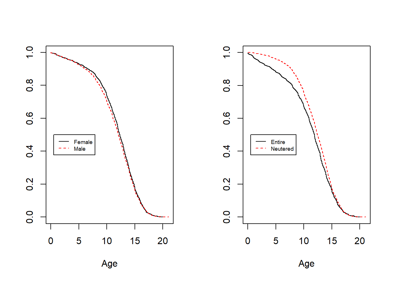
Figure 4.7: Survival Distributions by Sex and Being Neutered

Figure 4.8 shows survival distributions by breed where we plot distributions for the six most common breed types from Table 4.2, the remaining breeds are grouped into an “Other” category. The differences among survival distributions for different breeds are not surprising. Breeds may be a proxy for the size and weight of a dog; a larger dog like a Labrador has more risk than a smaller dog like a Jack Russell terrier, for example. The debate about whether mixed-breed dogs are generally healthier than purebred dogs is still ongoing among veterinary professionals. On the one hand, mixed breed dogs may be carriers of genetic mutations that lead to health issues; on the other hand, they are less likely than purebreds to develop the disorders themselves. As noted in NAIC (2019), it is common for insurance carriers to group the breeds into 10 to 12 rating categories, with each category assigned a rating factor.

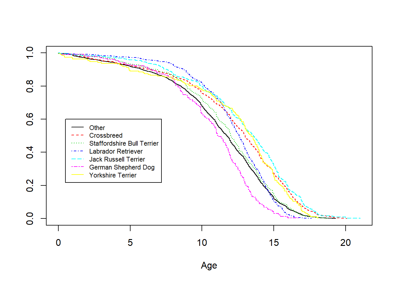
Figure 4.8: Survival Distributions by Breed

Table 4.3 summarizes the result of a (Cox proportional hazards) regression model fit using sex, being neutered, and breed as covariates. As suggested by Figure 4.7, the results suggest that sex is not an important variable given the other variables in the model. Further, there may be further opportunities to reduce the number of levels of the Breed variable as the Staffordshire Bull Terrier and Labrador Retriever distributions are not significantly different from the composite Other category.

R Code to Cox Regression Model Fit to Canine Survival

library(finalfit)
library(dplyr)

explanatory = c("Sex", "Neutered", "Breed2")
dependent = "Surv(AgeAtDeath)"
DogMort %>%
  coxphmulti(dependent, explanatory) %>%
  fit2df(condense = TRUE,
  metrics = FALSE, digits = c(2, 3,2),
  explanatory_name = "Risk Type", estimate_suffix = "  -- conf interval & p-value",
  estimate_name = "Exp(Coefficent)")  -> t2
t2[1] <- c("Male", "Neutered","Crossbreed","Staffordshire Bull Terrier", "Labrador Retriever", 
           "Jack Russell Terrier", "German Shepherd Dog", "Yorkshire Terrier")
knitr::kable(t2, align=c("l", "r"),caption="Fit of a Cox Proportional Hazards Model")

Table 4.3: Fit of a Cox Proportional Hazards Model

Risk Type	Exp(Coefficent) – conf interval & p-value
Male	1.04 (0.983-1.090, p=0.19)
Neutered	0.88 (0.837-0.929, p<0.01)
Crossbreed	0.65 (0.612-0.699, p<0.01)
Staffordshire Bull Terrier	0.93 (0.850-1.027, p=0.16)
Labrador Retriever	0.95 (0.860-1.044, p=0.28)
Jack Russell Terrier	0.57 (0.508-0.635, p<0.01)
German Shepherd Dog	1.44 (1.260-1.647, p<0.01)
Yorkshire Terrier	0.67 (0.581-0.779, p<0.01)

4.5.3 Cost of Care

With the estimated survival distribution, we can illustrate some of the types of calculations that a financial analyst might consider to quantify the cost of pet health insurance. These calculations are only for demonstration purposes; naturally, analysts that have access to detailed insurance costs will be able to sharpen our estimates. To begin, consider a male dog that is neutered belonging to the “Crossbreed” breed. Then, it is straightforward to determine one-year mortality rates, as summarized in Figure 4.9.

R Code to Convert Cox Regression Model Output to One-Year Mortality Rates

Cox_ph_1 <- coxph(Surv(AgeAtDeath) ~ Sex+Neutered+Breed2, data=DogMort)
sfit <- survfit(Cox_ph_1,newdata = data.frame(Sex="Male", Neutered="Neutered", Breed2 = "Crossbreed"))
#plot(sfit)
sx <- summary(sfit, times = 0:22)$surv
sx[1] = 1
qx <- 1 - sx[2:22]/sx[1:21]
qx[21] =1
plot(0:20,qx, xlab = "Age (x)", ylab = expression(q[x]), type = "both")

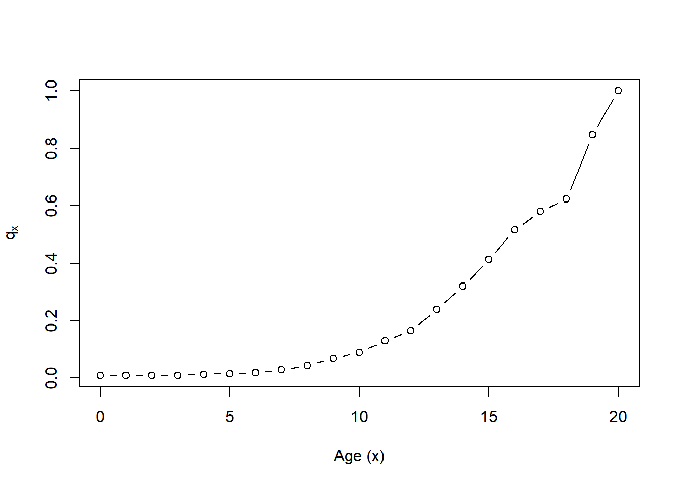
Figure 4.9: One Year Mortality Rates for a Neutered Male Crossbreed

From this estimated mortality, it straightforward to estimate financial costs, as illustrated in the following.

Example. Surgical Veterinary Care. Owning a pet can be expensive. According to the American Pet Products Association’s 2021-2022 National Pet Owners Survey, the basic annual expense for caring for a dog is 1480. This total cost consists of: Surgical vet (458), food (287), routine visit (242), kennel boarding (228), food treats (81), vitamins (81), toys 56), and groomer/grooming aids (47) (Source: III (2021)).

What about unanticipated costs? We estimate the actuarial present value associated with just one component, the surgical veterinary expenses, over a lifetime for a male dog aged \(x\) that has been neutered. As our baseline initial cost, we use 458 USD per year. Now, we know that expenses increase as a dog ages and we assume an annual increase of 11%. This may seem high but we are assuming a 3% increase due to inflation and an 8% real growth rate. The real growth rate is based on the rating scale from a large carrier where the age rating factor starts at 1 for pets ages 2-11 months and increases to 4.5 for pets over 20 years old, see Wilson (2020).

To compute the actuarial present value, we use the expression

\[ APV = ({\text {Initial Ann Cost}}) \sum_{k=0}^{\omega - x - 1} v^k ~(1.11)^k ~_k p_x . \]

This is based on equation (3.3) with the \(k\)-year survival probability \(~_kp_x\) and cost \(~_kC = ({\text {Initial Ann Cost}})~(1.11)^k\) \(= 458 ~(1.11)^k\). The discount factor is 3% for investments (so \(v=1/1.03\)) and the highest age is \(\omega = 22\). The calculations are summarized in Table 4.4. Not surprisingly, we see that older dogs (e.g., \(x=12\)) with a lower lifetime expectancy have a lower actuarial present value. In the same way, the German Shepard Dog has a higher mortality than the Crossbreed and so has a lower actuarial present value for the cost of care.

R Code to Create APVs from One-Year Mortality Rates

Cox_ph_1 <- coxph(Surv(AgeAtDeath) ~ Sex+Neutered+Breed2, data=DogMort)

DogAnn <- function(x=x, q.x=qx){
  Term <- length(q.x) - (x+1)
  kpx <- 1 
  APV  <- 0 
 if (Term>0){ for(k in 0:(Term-1)){ 
    if (k>1) {kpx <- kpx*(1-q.x[x+1+k])}
    APV  <- APV  + kpx *  (1/1.03)^k   *1.11^k *458
    }}
 return(APV)
  }

OneYearMortBreed <- function(Breed){
sfit <- survfit(Cox_ph_1,newdata = data.frame(Sex="Male", Neutered="Neutered", Breed2 = Breed))
sx <- summary(sfit, times = 0:22)$surv
sx[1] = 1
qx <- 1 - sx[2:22]/sx[1:21]
qx[21] =1
return(qx)
}

CostCare <- matrix(0, nrow = 2, ncol = 3)
qxCrossBreed <- OneYearMortBreed("Crossbreed")
CostCare[1,1] <- DogAnn(x=2, q.x=qxCrossBreed) 
CostCare[1,2] <- DogAnn(x=5, q.x=qxCrossBreed)
CostCare[1,3] <- DogAnn(x=12, q.x=qxCrossBreed)
qxGShepherd <- OneYearMortBreed("German Shepherd Dog")
CostCare[2,1] <- DogAnn(x=2, q.x=qxGShepherd) 
CostCare[2,2] <- DogAnn(x=5, q.x=qxGShepherd)
CostCare[2,3] <- DogAnn(x=12, q.x=qxGShepherd)

rownames(CostCare) <- c("Crossbreed","German Shepherd Dog" )
colnames(CostCare) <- c("x=2","x=5", "x=12" )

knitr::kable(CostCare, align=c("c", "c", "c"),caption="Actuarial Present Value of the Lifetime Cost of Surgical Vet Care", digits = 2)

Table 4.4: Actuarial Present Value of the Lifetime Cost of Surgical Vet Care

	x=2	x=5	x=12
Crossbreed	7382.5	4941.6	1741.2
German Shepherd Dog	5483.7	3546.1	1274.9

4.5.4 More on Pet Insurance Markets

History and Markets

As described in NAIC (2019), the first policy on a dog was issued in Sweden in 1924. In 1947, the first pet insurance policy was issued in the United Kingdom (UK). In Sweden and the UK, modern pet insurance policies are designed with the ability to cover pet medical costs and liability to third parties for the action of pets. In the U.S., the first pet policy was issued in 1982 that covered the dog that played Lassie on a popular U.S. television series, III (2021).

Pet insurance is more common in European countries than in the United States, with half of all pets in Sweden covered by pet health insurance. In the U.S., only about 1% of dogs and cats kept as pets are covered by pet insurance. As noted in Section 4.5.1, in part this is due to regulatory requirements. It may also be due to the longer history that pet insurance has enjoyed in parts of Europe.

Nonetheless, the pet insurance marketplace has been expanding rapidly in the U.S. with (premium) growth rates exceeding 10% for many years. According to a survey conducted by a large U.S. carrier, the fastest-growing form of distribution [of pet health insurance] is through an employee benefit package with about fifty percent of Fortune 500 companies offering pet insurance as an employee benefit, NAIC (2019).

Regulations and Economics

From a regulatory perspective, in the U.S. pet insurance falls under the property/casualty area of insurance because pets are, in effect, property. This places a bit of a burden on actuaries in that statutory reporting follows traditional property and casualty procedures whereas other aspects of pet insurance are more akin to (human) health practices; in the U.S., health insurance is regulated separately from property/casualty insurance.

Adverse selection, introduced in Section 4.3.2, is an important aspect of health insurance. It is natural for those in poor health to seek health insurance because they can reasonably expect higher costs. This can be a problem for insurers if they are unaware of the poor health conditions (we called this “information asymmetry” in Section 4.3.3). In many jurisdictions such as the U.S., there are rules that prohibit insurers from denying coverage for pre-existing (typically poor health) conditions. In contrast, for pet insurance animals with pre-existing conditions are generally not eligible for coverage. This avoids, for example, a situation in which a pet owner could find out his or her dog has cancer or another condition requiring expensive treatment and then tries to buy insurance to cover it.

Pet insurers also need to be aware of another type of information asymmetry, moral hazard, where the presence of the insurance cover alters survival probabilities (recall Section (Sec:AsymmericInfo)). Moral hazard is not necessarily bad. In fact, perhaps the primary reason that veterinarians promote pet health insurance is so that they may advise pet owners on appropriate medical treatments and not be hampered by cost concerns. For example, sometimes veterinarians feel they must offer euthanasia as an option because the animal may be suffering from a treatable condition but the client may be unable to afford the proposed treatment due to lack of pet insurance, a situation termed economic euthanasia.

4.6 Disability Income Insurance

---

In this section, you learn how to:

• Describe disability income insurance.
• Analyze disability recovery, a contingent event that is not based on human mortality.
• Demonstrate the impact of selection on actuarial present values of disability income insurance.

---

4.6.1 Introduction to Disability Income Insurance

Disability income insurance is a contract designed to provide a regular income, such as monthly, to an individual if he or she is prevented by sickness or injury from working. Policies are available on an individual basis, through membership in a group such as sponsored by an employer, and through public government sponsored insurance. The data that we consider are from the U.S. Social Security Disability Income program, Zayatz (2015). Because disability income provides benefits to those unable to work, it is not designed to be a substitute for a retirement benefit and so is usually available up to a fixed term or age, such as ceasing at age 65 as in our illustrative example.

Like annuity benefits introduced in Section 3.3, the benefit is paid periodically until a random event time. However, for a life annuity, the payment stops when the policyholder dies (a sad event). In contrast, for a disability income policy, we first focus on the payment stopping when someone recovers from disability (a happy event).

Contingent payment techniques can be employed for general event times that need not be tied to human mortality. Naturally, there are a few caveats to this important message. For example, both life annuities and disability income may be limited by a fixed term or age. Further, as we will see, disability income may cease upon the sooner of recovery or death, another type of event time.

4.6.2 Disability Recovery Rates

To better appreciate how often policyholders recover from disability, Figure 4.10 shows male rates \(q_x^r\) from the U.S. Social Security Disability Income program (Zayatz (2015), Table 14A). These data are organized in Appendix Section 8.7. The \(r\) superscript reminds us that these are recovery, not mortality, rates. The solid black line, denoted as Select=0, is for individuals who met program qualifications for disability benefits and then recovered from their disability within a year. As suggested in the figure, except for age less than about 22, this experience is very similar to individuals who had been in the program for two years, Select=2. The other four lines represent greater number of years of selection (4, 6, 8, and an “ultimate” column); visually, they seem similar to one another. This figure demonstrates the importance of the select effect and is consistent with medical selection in life insurance that we saw in Section 4.3.2. In both cases, recent admission to a program or policy can influence the “event time” experience.

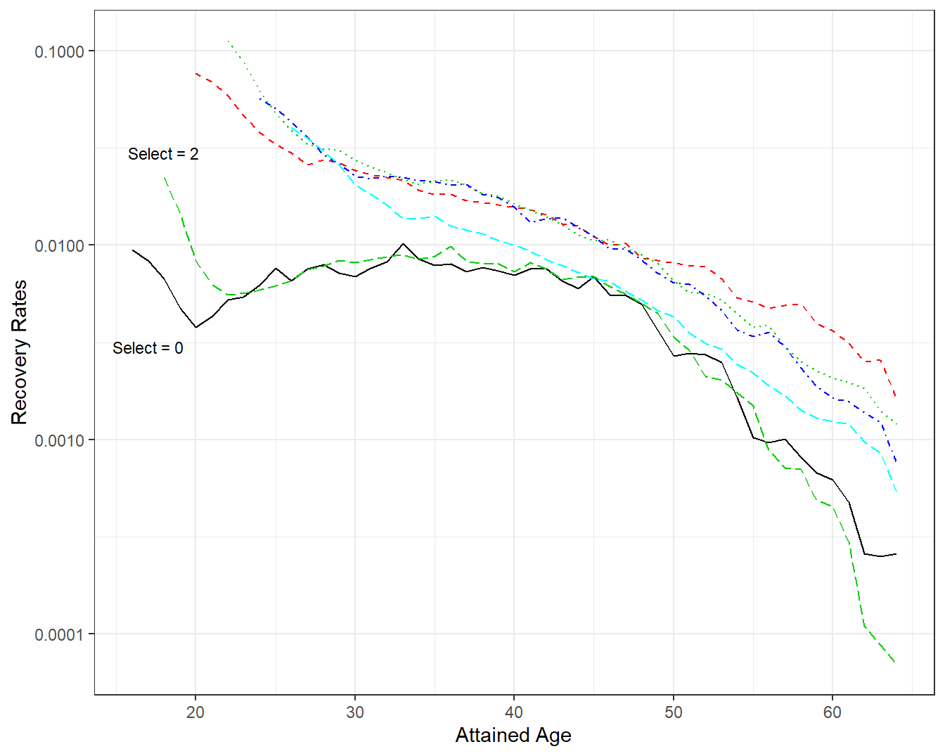
Figure 4.10: Disability Recovery Rates by Attained Age and Select Period. A plot of recovery rates \(q_x^r\) by attained age \(x\). Each line represents a different select period. The lines for select 0 and 2 are similar, other lines are also similar, suggesting that selection effects have worn out beginning at select = 4.

As in Section 2.1.1, another way of looking at event times is by following cohorts of individuals. Figure 4.11 follows recovery rates for several cohorts; this figure emphasizes that annual probabilities of recovery decline with advancing age. As noted in Zayatz (2015), the early year probability of recovery patterns are attributed to the scheduling of continuing disability reviews. For example, where medical improvement is expected, the review is scheduled for 6 to 24 months following the most recent disability decision. Where medical improvement is not expected, the review is scheduled between 5 and 7 years later.

These patterns are most evident in the cohort depicted by the bold solid black line that follows males who entered the disability program at age 16. This is the youngest cohort in the data set; it has the least amount of experience and so is the most uncertain. From Figure 4.11, we see a very large spike in recovery rates after five or six years in the program. This spike is also evident in cohorts that entered at ages 21 and 26 although on a smaller scale. The jump in recovery rates beginning at Cohort=31 and on is still evident but on a much lower scale.

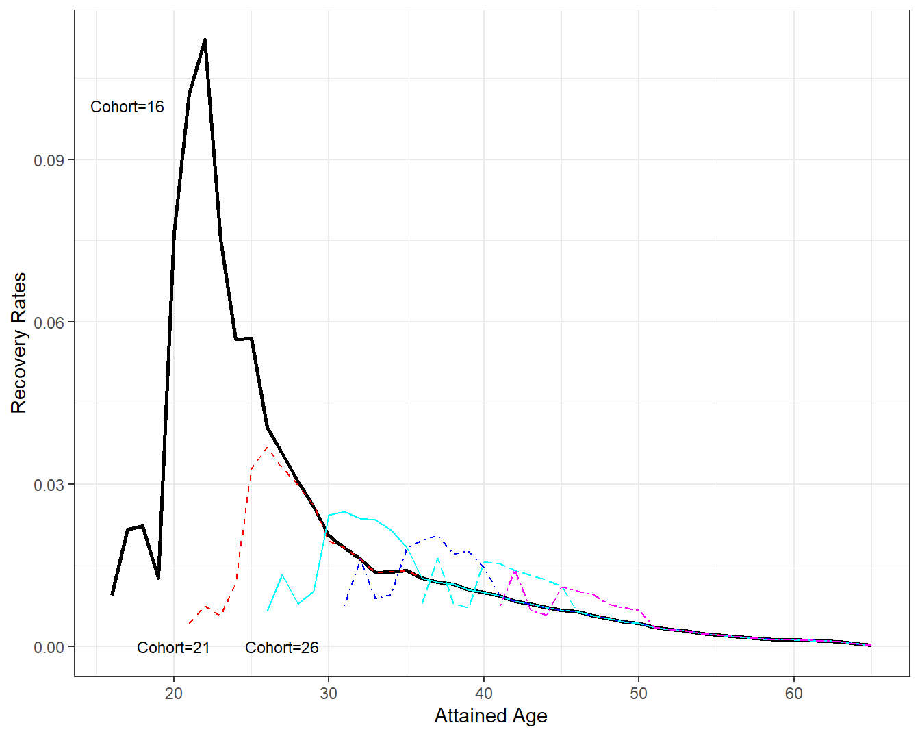
Figure 4.11: Disability Recovery Rates by Attained Age and Cohort. A plot of recovery rates \(q_x^r\) by attained age \(x\). Each line represents a different cohort. The cohort first receiving disability benefits at age 16 show a strong recovery rate about five years later. This effect is also evident, although not as pronounced, in cohorts 21 and 26. Recovery rates seem to dampen as age (both cohort and attained) increases.

4.6.3 Actuarial Present Values of Disability Income

To get a sense of the benefit to an individual, and the cost to the program, we can compute actuarial present values. Calculation of the actuarial present value is that same as the term life annuity introduced in Section 3.3.2 in that we assume the benefit terminates at age 65. Further, instead of probability of death we now use probability of recovery from disability (and hence exiting the program).

Using an assumed \(i=\) 4 percent interest rate, Figure 4.12 summaries annuity calculations by attained age for several different cohorts. These annuity values assume a payment of 1 at the beginning of the year if one is in the program; for perspective, as reported in Zayatz (2015), in 2013 (the year of the study) disability income worker beneficiaries received approximately 14,000 USD per year.

Although there are some differences at younger cohorts and attained ages, Figure 4.12 shows remarkable agreement among cohorts beginning about age 30. In the figure, the thick dashed blue line marks annuity values for the Cohort=31; all annuity values are similar to this line. We can interpret this to mean that the actuarial present value depends on the attained age for 30 and above, not the cohort representing when an individual first entered the program.

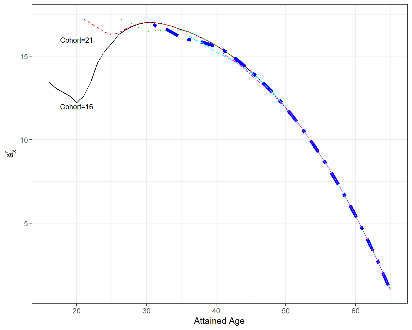
Figure 4.12: Annuities by Attained Age and Cohort. A plot of annuities \(ä_x^r\) by attained age \(x\). Each line represents a different cohort. The first two cohorts plotted first receiving disability benefits at age 16 and 21 differ in the early annuity values. Beginning at attained age 30, all annuity values appear to be qualitatively similar. The thick dashed blue line marks annuity values for the cohort=31.

Figure 4.13 supplements that actuarial present values by providing an analysis for female workers. The top two lines of the figure show that male and female actuarial present values are virtually indistinguishable when the event time is recovery. Based on our prior work, this figure only presents Cohort=31.

The lower two lines in Figure 4.13 consider the event time to be the sooner of recover and death for males and females, respectively. That is, a worker may leave the program due to recover from disability as well as death. So, when computing actuarial present values, this broader measure of exiting the program is used. The lower two lines show that female annuities are above male annuities; this is consistent with our prior observations that females generally live longer then males.

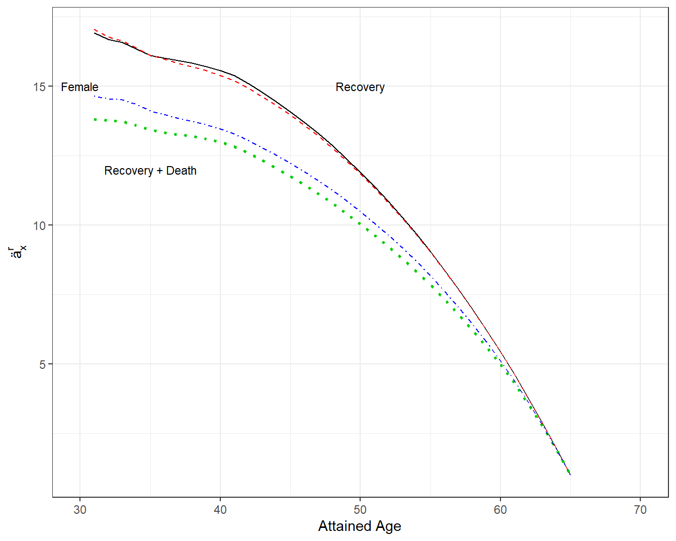
Figure 4.13: Annuities by Attained Age, Gender and Type of Departure. A plot of annuities \(ä_x^r\) by attained age \(x\). The top two lines are represent departing from the disability program via recovery from disability. The two lines are for male and female and are virtually indistinguishable. The bottom two lines represent departing from the disability program via recovery from disability or by death. Female annuities are above male annuities (in that females generally live longer then males).

4.6.4 More on Disability Income Insurance

This brief introduction to disability income focused on demonstrating an important application where contingent payment methods need not use mortality as the time to an event. Because of its brevity, we have omitted many important attributes of disability income such as a waiting time for benefit eligibility, the role of monthly payments, differences among individual, group, and public programs, as well as features of different international marketplaces. For a deeper dive into this fascinating topic, see Haberman and Pitacco (2018).

In particular, we have not yet addressed the cost of becoming disabled. What we have done is provide actuarial present values of the benefit of a disability insurance program. However, for a worker, we have not yet described the probability of being disabled. More generally, in a worker’s lifetime, someone can start as an active worker, become disabled, and as we have seen, that the person may quickly recover from the disability and then re-enter the work force. This pattern of switching statuses between between healthy and working and disabled and receiving benefits, and costs associated with each status, is the topic of Chapter 7 on multiple state modeling.

Section Structure Discussions

Easy to include moral hazard into disability income insurance discussions….

References

Haberman, Steven, and Ermanno Pitacco. 2018. Actuarial Models for Disability Insurance. Routledge.

Hoffman, Christy L, Melissa Thibault, and Julie Hong. 2021. “Characterizing Pet Acquisition and Retention During the Covid-19 Pandemic.” Frontiers in Veterinary Science 8.

III. 2021. “Facts + Statistics: Pet Ownership and Insurance.” In. Insurance Information Institute. https://www.iii.org/fact-statistic/facts-statistics-pet-ownership-and-insurance.

Malloy, Michael G. 2018. “A Policy for Fluffy: Pet Insurance Is a Small Industry-but It’s Poised for Big Growth in the U.s.” Contingencies. https://contingencies.org/a-policy-for-fluffy-pet-insurance-is-a-small-industry-but-its-poised-for-big-growth-in-the-u-s-%E2%80%83/.

NAIC. 2019. “A Regulators Guide to Pet Insurance.” In. National Association of Insurance Commissioners. https://content.naic.org/sites/default/files/publication-pin-op-pet-insurance.pdf.

OECD. 2020. “Insurance Statistics Yearbook.” Paris. Organization for Economic Co-operation; Development (OECD). https://stats.oecd.org/Index.aspx?DatasetCode=INSIND.

Pegram, Camilla, Carol Gray, Rowena MA Packer, Ysabelle Richards, David B Church, Dave C Brodbelt, and Dan G O’Neill. 2021a. “Proportion and Risk Factors for Death by Euthanasia in Dogs in the Uk.” Scientific Reports 11 (1): 1–12.

Pegram, Camilla, Carol Gray, Rowena MA Packer, Ysabelle Richards, David B Church, Dave C Brodbelt, and Dan G O’Neill. 2021b. “Proportion and Risk Factors for Death by Euthanasia in Dogs in the Uk– Supporting Data.” https://researchonline.rvc.ac.uk/id/eprint/13486/.

Verteramo Chiu, Leslie J, Jie Li, Guillaume Lhermie, and Casey Cazer. 2021. “Analysis of the Demand for Pet Insurance Among Uninsured Pet Owners in the United States.” Veterinary Record, e243.

Wilson, Kimberly L. 2020. “Underwriting Criteria, Practices, and Tools of Pet Health Insurance Companies.” Connecticut Insurance Law Journal 27 (1): 359–405.

Zayatz, Tim. 2015. “Social Security Disability Insurance Program Worker Experience.” Actuarial Study 123. https://ai.ssa.gov/OACT/NOTES/pdf_studies/study123.pdf.