Chapter 9 Appendix: Conventions for Notation

Chapter Preview. Life Contingencies employs widely accepted statistical concepts and tools. Thus, the notation should be consistent with standard usage employed in probability and mathematical statistics. See, for example, (Halperin, Hartley, and Hoel 1965) for a description of one standard.

9.1 Actuarial Notation

Here is a list of commonly used actuarial symbols and functions, including the latex code that we use to generate them.

9.1.1 Life Table Symbols

\(\require{enclose}\)

\[ {\small \begin{array}{cll} \hline \textbf{Symbol} & \textbf{Latex code} & \textbf{Description} \\ \hline \ell_{x} & \verb|\| \tt{ell}\_\{\tt{x}\} & \text{Expected number of lives at age } x \\ \ell_{[x]} & \backslash\tt{ell}\_\{ [\tt{x}]\} & \text{Expected number of lives at select age } x \\ _{t}p_{x} & ~ \_\{ \tt{t} \} \tt{p} \_ \{\tt{x}\} & \text{Probability that a life aged } x \text{ survives }t \text{ years} \\ _{t}p_{[x]} & ~ \_\{ \tt{t} \} \tt{p} \_ \{ [\tt{x}]\}\} & \text{Probability that a select life aged } x \text{ survives }t \text{ years} \\ \mathring{e}_{x} & \backslash\tt{mathring\{e\}} \_ \{ x\} & \text{Complete expectation of life at age } x \\ \mathring{e}_{x:{\enclose{actuarial}{n}}} & \backslash\tt{mathring\{e\}} \_ \{ x:\{\backslash enclose\{actuarial\}\{n\}\}\} & \text{Complete expectation of life at age } x \text{ for the next } n \text{ years} \\ \hline \end{array} } \]

9.1.2 Life Insurance Symbols

\[ {\small \begin{array}{cll} \hline \textbf{Symbol} & \textbf{Latex code} & \textbf{Description} \\ \hline A_{x} & \tt{A} \_ \{\tt{x}\} & \text{APV of a discrete whole life insurance to } (x) \\ \bar{A}_{x} & \backslash \tt{bar} \{\tt{A}\} \_ \{\tt{x}\} & \text{APV of a continuous whole life insurance to } (x) \\ A^{(m)}_{x} & \tt{A} \verb|^| \tt{\{(m)\}}\_ \{\tt{x}\} & \text{APV of a whole life insurance payable at end of } m\text{-th of the year of death of } (x) \\ _{n}E_{x} & ~ \_\{ \tt{n} \} \tt{E} \_ \{\tt{x}\} & \text{APV of an } n\text{-year pure endowment to } (x) \\ {A}_{x:\enclose{actuarial}{n}}^{\quad 1} & \{\tt{A}\} \_ \{ x:\{\backslash enclose\{actuarial\}\{n\}\}\} \verb|^| \{\backslash \tt{quad} \ 1\} & \text{APV of an } n\text{-year term insurance to } (x) \\ {A}_{x:{\enclose{actuarial}{n}}} & \{\tt{A}\} \_ \{ x:\{\backslash enclose\{actuarial\}\{n\}\}\} & \text{APV of an } n\text{-year endowment insurance to } (x) \\ _{n|}{A}_{x} & ~ \_\{ \tt{n|} \} \{\tt{A}\_\{x\}\} & \text{APV of an } n\text{-year deferred life insurance to } (x) \\ {A}_{x:\enclose{actuarial}{n}}^{\space 1} & \{\tt{A}\} \_ \{ x:\{\backslash enclose\{actuarial\}\{n\}\}\} \verb|^| \{\backslash \tt{space} \ 1\} & \text{APV of an } n\text{-year term insurance to } (x) \\ \hline \end{array} } \]

9.1.3 Annuity Certain and Life Annuity Symbols

\[ {\small \begin{array}{cll} \hline \textbf{Symbol} & \textbf{Latex code} & \textbf{Description} \\ \hline a_{\enclose{actuarial}{n}} & \tt{a}\_\{\backslash \tt{enclose}\{actuarial\}\{\tt{n}\}\} & n\text{-year annuity certain-immediate} \\ \ddot{a}_{\enclose{actuarial}{n}} & \backslash\tt{ddot}\_\{\tt{a}\_\{\backslash \tt{enclose}\{actuarial\}\{\tt{n}\}\} & n\text{-year annuity certain-due} \\ \ddot{a}^{(m)}_{\enclose{actuarial}{n}} & \backslash\tt{ddot} \verb|^| \tt{\{(m)\}}\_\{\tt{a}\_\{\backslash \tt{enclose}\{actuarial\}\{\tt{n}\}\} & n\text{-year annuity certain-due payable } m\text{-thly} \\ _{m|}\ddot{a}_{\enclose{actuarial}{n}} & ~ \_\{ \tt{m|} \} \backslash\tt{ddot}\_\{\tt{a}\_\{\backslash \tt{enclose}\{actuarial\}\{\tt{n}\}\} & m\text{-year deferred } n\text{-year annuity certain-due} \\ a_{x} & \tt{a}\_\{x\} & \text{APV of a whole life annuity immediate to } (x) \\ \ddot{a}_{x} & \backslash\tt{ddot}\{\tt{a}\}\_\{x\} & \text{APV of a whole life annuity due to } (x) \\ a^{(m)}_{x} & \tt{a} \verb|^| \tt{\{(m)\}}\_\{x\} & \text{APV of a life annuity immediate to } (x) \text{ payable } m\text{-thly} \\ \ddot{a}^{(m)}_{x} & \backslash\tt{ddot}\{\tt{a}\} \verb|^| \tt{\{(m)\}}\_\{x\} & \text{APV of a life annuity due to } (x) \text{ payable } m\text{-thly} \\ _{n|}\ddot{a}_{x} & ~ \_\{ \tt{n|} \} \backslash\tt{ddot}\_\{\tt{a}\_\{x\}\} & \text{APV of an } n\text{-year deferred life annuity due to } (x) \\ \ddot{a}_{x:{\enclose{actuarial}{n}}} & \backslash\tt{ddot\{a\}} \_ \{ x:\{\backslash enclose\{actuarial\}\{n\}\}\} & \text{APV of an } n\text{-year life annuity due to } (x) \\ \ddot{a}^{(m)}_{x:{\enclose{actuarial}{n}}} & \backslash\tt{ddot\{a\}} \verb|^| \tt{\{(m)\}} \_ \{ x:\{\backslash enclose\{actuarial\}\{n\}\}\} & \text{APV of an } n\text{-year life annuity due to } (x) \text{ payable } m\text{-thly} \\ \hline \end{array} } \]

Not sure if necessary to say \(APV\) (actuarial present value)

9.2 Halo System

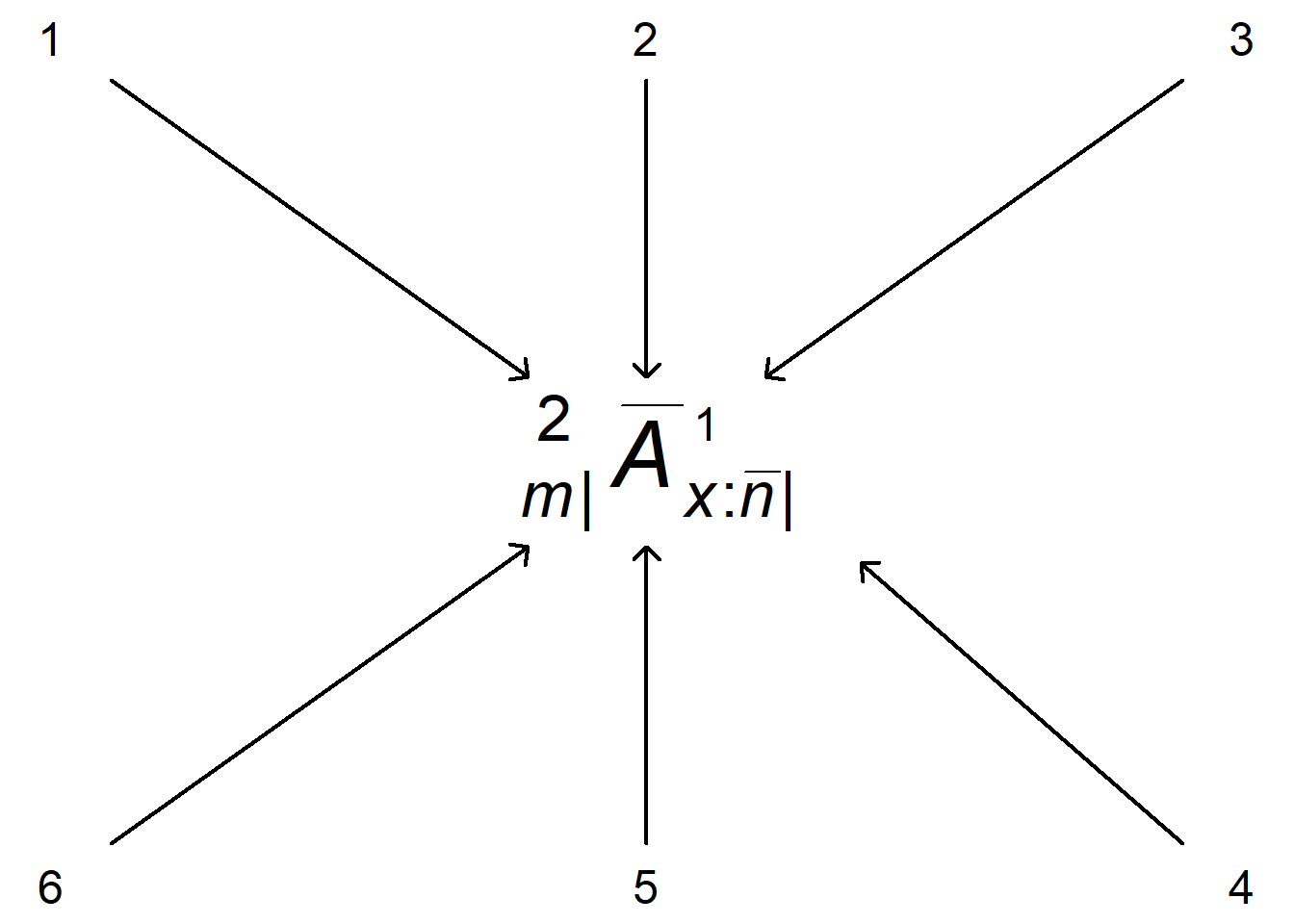
Figure 9.1: Halo System: Example of an Actuarial Symbol. Source: This is adapted from the Wikipedia page Actuarial Notation.

---

Legend:

• 1 - the “2” means double the force of interest
• 2 - the bar implies continuous, or payments at the moment of death. No bar, or blank, signifies payment at the end of the year. For annuities, could use a double dot that signifies payments at the beginning of the year.
• 3 - the “1” denotes a temporary, or term, payment. Paid if \(x\) within \(n\) years
• 4 - contract issued to a life aged \(x\) and lasts for at most \(n\) years.
• 5 - the “A” signifies it is an insurance (“assurance”) contract. Could also be a lower case \(a\) that would signify an annuity contract.
• 6 - deferred m years

Note: It is sometimes helpful to put a space before the pre-subscript like \(\frac{\ell_{[x]+t}}{\ell_{[x]}} = ~_{t}p_{[x]}\). Else you get this awkward \(\frac{\ell_{[x]+t}}{\ell_{[x]}} = _{t}p_{[x]}\).

\[ Y = \begin{cases} 1 + v + v^2 + \cdots + v^K = \ddot{a}_{\enclose{actuarial}{K+1}}, K=0,1,\ldots,n-1 \\ 1 + v + v^2 + \cdots + v^{n-1} = \ddot{a}_{\enclose{actuarial}{n}}, K \ge n \end{cases} \] Note.

• For the html version of the text, we are using the STACK system; in particular, see their actuarial notation page.
• This does not appear to work for the pdf version, at least with R-Studio. The latex package actuarialangle provides a substitute. To make this happen, in our latex header .tex page, we have the following bit of code

%  Something for the Actuarial Angle package
\usepackage{actuarialangle}
\newcommand{\enclose}[1]{\actuarialangle} 

9.3 General Conventions

• Random variables are denoted by upper-case italicized Roman letters, with \(X\) or \(Y\) denoting a claim size variable, \(N\) a claim count variable, and \(S\) an aggregate loss variable. Realizations of random variables are denoted by corresponding lower-case italicized Roman letters, with \(x\) or \(y\) for claim sizes, \(n\) for a claim count, and \(s\) for an aggregate loss.
• Probability events are denoted by upper-case Roman letters, such as \(\Pr(\mathrm{A})\) for the probability that an outcome in the event ‘’A’’ occurs.
• Cumulative probability functions are denoted by \(F(z)\) and probability density functions by the associated lower-case Roman letter: \(f(z)\).
• For distributions, parameters are denoted by lower-case Greek letters. A caret or ‘’hat’’ indicates a sample estimate of the corresponding population parameter. For example, \(\hat{\beta}\) is an estimate of \(\beta\) .
• The arithmetic mean of a set of numbers, say, \(x_1, \ldots, x_n\), is usually denoted by \(\bar{x}\); the use of \(x\), of course, is optional.
• Use upper-case boldface Roman letters to denote a matrix other than a vector. Use lower-case boldface Roman letters to denote a (column) vector. Use a superscript prime ’‘\(\prime\)’’ for transpose. For example, \(\mathbf{x}^{\prime} \mathbf{A} \mathbf{x}\) is a quadratic form.
• Acronyms are to be used sparingly, given the international focus of our audience. Introduce acronyms commonly used in statistical nomenclature but limit the number of acronyms introduced. For example, pdf for probability density function is useful but GS for Gini statistic is not.

9.4 Abbreviations

Here is a list of abbreviations that we adopt. We italicize these acronyms. For example, we can discuss the goodness of fit in terms of the AIC criterion.

\[ \begin{array}{ll} \hline \textbf{Symbol} & \textbf{Description} \\ \hline AIC & \text{Akaike information criterion} \\ BIC & \text{(Schwarz) Bayesian information criterion} \\ cdf & \text{cumulative distribution function} \\ df & \text{degrees of freedom} \\ iid & \text{independent and identically distributed} \\ GLM & \text{generalized linear model} \\ mle & \text{maximum likelihood estimate/estimator}\\ ols & \text{ordinary least squares} \\ pdf & \text{probability density function} \\ pmf & \text{probability mass function} \\ \hline \end{array} \]

9.5 Common Statistical Symbols and Operators

Here is a list of commonly used statistical symbols and operators, including the latex code that we use to generate them (in the parens).

\[ \begin{array}{cl} \hline \textbf{Symbol} & \textbf{Description} \\ \hline I(\cdot) & \text{binary indicator function (}I\text{). For example, }I(A) \text{ is one if an outcome in event} \\ & \ \ \ \ \ A \text{ occurs and is 0 otherwise.} \\ \Pr(\cdot) & \text{probability }(\backslash{\tt{Pr}}) \\ \mathrm{E}(\cdot) & {\text{expectation operator }} (\backslash{\tt{mathrm\{E\}}}). {\text{ For example, }} \mathrm{E}(X)=\mathrm{E}~X {\text{ is the }} \\ & \ \ \ \ \ {\text{expected value of the random variable }}X,{\text{ commonly denoted by }}\mu. \\ \mathrm{Var}(\cdot) & \text{variance operator }(\backslash{\tt{mathrm\{Var\}}}). \text{ For example, } \mathrm{Var}(X)=\mathrm{Var}~X\text{ is the} \\ & \ \ \ \ \ \text{ variance of the random variable } X, \text{commonly denoted by } \sigma^2. \\ \mu_k = \mathrm{E}~X^k & \text{kth moment of the random variable X. For }k\text{=1, use }\mu = \mu_1. \\ \mathrm{Cov}(\cdot,\cdot) & \text{covariance operator } (\backslash{\tt{mathrm\{Cov\}}}).\text{ For example, } \\ & \ \ \ \ \ \mathrm{Cov}(X,Y)=\mathrm{E}\left\{(X -\mathrm{E}~X)(Y-\mathrm{E}~Y)\right\} =\mathrm{E}(XY) -(\mathrm{E}~X)(\mathrm{E}~Y)\\ & \ \ \ \ \ \text{ is the covariance between random variables }X\text{ and }Y. \\ \mathrm{E}(X | \cdot) & \text{conditional expectation operator. For example, }\mathrm{E}(X |Y=y) \text{ is the}\\ & \ \ \ \ \ \text{ conditional expected value of a random variable }X\text{ given that }\\ & \ \ \ \ \ \text{ the random variable }Y\text{ equals y. }\\ \Phi(\cdot) & \text{standard normal cumulative distribution function }(\backslash{\tt{Phi}})\\ \phi(\cdot) & \text{standard normal probability density function }(\backslash{\tt{phi}})\\ \sim & \text{means is distributed as }(\backslash{\tt{sim}}). \text{ For example, }X\sim F \text{ means that the } \\ & \ \ \ \ \ \text{random variable } X \text{ has distribution function }F. \\ se(\hat{\beta}) & \text{standard error of the parameter estimate }\hat{\beta} ~ (\backslash{\tt{hat\{}}\backslash{\tt{beta\}}}), \text{ usually }\\ & \ \ \ \ \ \text{ an estimate of the standard deviation of }\hat{\beta},\text{ which is }\sqrt{Var(\hat{\beta})}. \\ H_0 & \text{null hypothesis} \\ H_a \text{ or }H_1 & \text{alternative hypothesis} \\ \hline \end{array} \]

9.6 Common Mathematical Symbols and Functions

Here is a list of commonly used mathematical symbols and functions, including the latex code that we use to generate them (in the parens).

\[ \begin{array}{cll} \hline \textbf{Symbol} & \textbf{Latex code} & \textbf{Description} \\ \hline \equiv & \backslash\tt{equiv} & \text{identity, equivalence} \\ \implies & \backslash\tt{implies} & \text{implies} \\ \iff & \backslash\tt{iff} & \text{if and only if} \\ \to, \longrightarrow & \backslash\tt{to}, \backslash\tt{longrightarrow} & \text{converges to} \\ \mathbb{N} & \backslash\tt{mathbb\{N\}} & \text{natural numbers }1,2,\ldots \\ \mathbb{R} & \backslash\tt{mathbb\{R\}} & \text{real numbers} \\ \in & \backslash\tt{in} & \text{belongs to} \\ \notin & \backslash\tt{notin} & \text{does not belong to} \\ \subseteq & \backslash\tt{subseteq} & \text{is a subset of} \\ \subset & \backslash\tt{subset} & \text{is a proper subset of} \\ \cup & \backslash\tt{cup} & \text{union} \\ \cap & \backslash\tt{cap} & \text{intersection} \\ \emptyset & \backslash\tt{emptyset} & \text{empty set} \\ A^{c} & & \text{complement of }A \\ g*f & & \text{convolution }(g*f)(x)=\int_{-\infty}^{\infty}g(y)f(x-y)dy \\ \exp & \backslash\tt{exp} & \text{exponential} \\ \log & \backslash\tt{log} & \text{natural logarithm }\\ \log_a & & \text{logarithm to the base }a \\ ! & & \text{factorial} \\ \text{sgn}(x) & \backslash\tt{sgn} & \text{sign of x} \\ \lfloor x\rfloor & \backslash\tt{lfloor}, \backslash\tt{rfloor} & \text{integer part of x, that is, largest integer }\leq x \\ |x| & & \text{absolute value of scalar }x \\ \varGamma(x) & \backslash\tt{varGamma} & \text{gamma (generalized factorial) function},\\ & & \text{satisfying }\varGamma(x+1)=x\varGamma(x) \\ B(x,y) & & \text{beta function, }\varGamma(x)\varGamma(y)/\varGamma(x+y) \\ \hline \end{array} \]

9.7 Further Readings

To make connections to other literatures, see (Abadir and Magnus 2002) for a summary of notation from the econometrics perspective. This reference has a terrific feature that many latex symbols are defined in the article. Further, there is a long history of discussion and debate surrounding actuarial notation; see (Boehm et al. 1975) for one contribution.

References

Abadir, Karim, and Jan Magnus. 2002. “Notation in Econometrics: A Proposal for a Standard.” The Econometrics Journal 5 (1): 76–90.
Boehm, C, J Engelfriet, M Helbig, A IM Kool, P Leepin, E Neuburger, and AD Wilkie. 1975. “Thoughts on the Harmonization of Some Proposals for a New International Actuarial Notation.” Blätter Der DGVFM 12 (2): 99–129.
Halperin, Max, Herman O Hartley, and Paul G Hoel. 1965. “Recommended Standards for Statistical Symbols and Notation: Copss Committee on Symbols and Notation.” The American Statistician 19 (3): 12–14.