Chapter 3 Basic Life Contingent Benefits
\(\require{enclose}\)
Chapter Preview. This chapter introduces the modeling of life contingent benefits, integrating the material from the previous chapter with basic concepts from financial mathematics. In contrast to benefits that are certain to be paid at specified periods, life contingent benefits have the additional complexity that the timing of payments is uncertain and are contingent upon either the survival or mortality of one or more lives. In this chapter we introduce the calculations of the present values of these contingent benefits, along with associated notation.
In this chapter we assume that benefits are paid at annual times. Benefits paid continuously or more frequently than annual time, along with other extensions, are considered in Chapter 4.
3.1 Valuation of Cash Flows under Uncertainty
In this section, you learn how to:
- Express a random cash flow as a product of a discount rate, a potential cash flow amount, and an indicator for the occurrence the cash flow
- Determine moments of the sum of random cash flows, emphasizing the mean and variance
- Compute these moments use a spreadsheet approach as well as
Rstatistical software
Imagine a financial system with a cash flow of known value \(_tC\) occurring in \(t\) years from now. If we assume the spot rate of interest is \(_ti\) per annum effective, then the present value (\(PV\)) of this cash flow is:
\[ PV = ~_tC ~(1+{_ti})^{-t}=~_tC ~ v^t . \tag{3.1} \]
Let us now introduce uncertainty into this system. Uncertainty might be in terms of the interest rate, the values of the amount, or the timing. In this chapter we assume spot rate \(_ti\) is known and that, if a cash flow occurs, the amount \(_tC\) is known (as we will see, it is typically set in an insurance contract). The uncertainty is in the timing, that is, whether a cash flow occurs which is represented by an indicator variable. More precisely, we assume that at each time \(t\) there is a Bernoulli random variable \(_tB\) that is one if a (non-zero) cash flow occurs and 0 otherwise. With this notation, at time \(t\), the present value of the random cash flow is \(v^t \times ~_tC \times ~_tB\).
To simplify matters so that we can focus on the foundations, this chapter assumes that timing \(t\) can only take on non-negative discrete integer values, denoted as \(k \in \{0,1,2,3, \ldots\}\). This system is illustrated on a timeline in Figure 3.1.
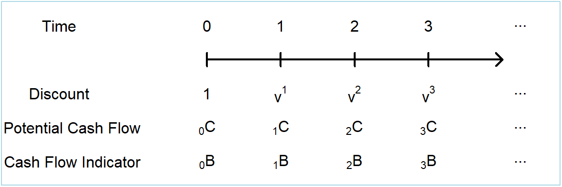
Figure 3.1: Timeline of cash flows with uncertainty
The present value \(PV\) is the sum of a number of discrete random variables that we can express as
\[ \begin{array}{l} PV = \sum_{k=0}^{\infty} v^k ~_kC~_kB~ .\\ \end{array} \tag{3.2} \]
There is no harm in letting the upper limit of the sum be infinity although for our applications it will be typically limited to a finite sum by contractual provisions in \(~_kC\) or human mortality through \(_kB\).
3.1.1 Moment Calculations
Because \(PV\) is a random variable, we are able to summarize certain aspects of its distribution by calculating moments such as the mean and variance. Given that \(_kC\) and \(v^k\) are known, we can calculate the expected present value as follows:
\[ \boxed{ \begin{array}{ll} \mathrm{E}(PV) &= \mathrm{E} \left[ \sum_{k=0}^{\infty} ~_kC~_kB~ v^k \right] \\ &= \sum_{k=0}^{\infty} ~_kC~ v^k ~\Pr(_kB = 1) . \end{array} } \tag{3.3} \]
In this expression, we use the fact that the mean of a Bernoulli random variable equals the probability of being a one, that is, \(\mathrm{E}(_kB) = 0 \times \Pr(_kB = 1)\) \(+ 1 \times \Pr(_kB = 1) = \Pr(_kB = 1)\). The calculation in equation (3.3) does not depend on the dependence relationships among the \(_kB\) random variables; sums of expectations of random variables are not affected by correlations between random variables.
Calculation of the variance of the present value does depend on the correlation among the cash flow indicators \(_kB\). For life contingent applications, we focus on three cases of interest:
- cash flow indicators are mutually independent,
- cash flow indicators are a function of the death of an individual, and
- cash flow indicators are a function of the survival of an individual.
For the first situation, you can think of classic gambling situations where the outcome of one game does not affect another. This situation is of less interest to us but does serve as useful benchmark. In this case, the variance of the present value is
\[ \mathrm{Var}(PV) = \sum_{k=0}^{\infty} ~_kC^2 ~v^{2k} ~\Pr(_kB=1)[1-\Pr(_kB=1)] . \]
In this expression, we use the fact that the variance of a Bernoulli random variable is \(\mathrm{Var}(_kB) = \Pr(_kB = 1)[1-\Pr(_kB=1)]\).
In the second case, cash flow indicators are a function of death in the period that can be represented by an indicator function \(I(K_{\bf{x}}=k)\). Recall from Chapter 2 that we defined the random variable \(K_{\bf{x}}\) as being the curtate death time (measured in years from the current time) for a life with set of attributes \(\bf{x}\). In our models, death can occur at most one time (no necromancy) and so for example, \(I(K_{\bf{x}}=10)I(K_{\bf{x}}=15) = 0\), that is, death in the \(10^{th}\) period and the \(15^{th}\) period cannot both occur. This means that \(_sB \times ~_rB =0\) for \(r \ne s\) and
\[ \begin{array}{l} PV^2 = \sum_{k=0}^{\infty} v^{2k} ~_kC^2~_kB~, \\ \end{array} \]
because all the cross-products are zero and an indicator variable squared is simply the indicator variable (\(_kB^2 = ~_kB\)). From this and the \(\mathrm{Var}(PV)\) \(= \mathrm{E}(PV^2) - [\mathrm{E}(PV)]^2\) formula, we have
\[ \mathrm{Var}(PV) = \sum_{k=0}^{\infty} ~_kC^2 ~v^{2k} ~\Pr(_kB=1) - [\mathrm{E}(PV)]^2 . \tag{3.4} \]
Single event cash flows typically occur when modeling life insurance benefits, the topic of Section 3.2.
In the third case, cash flow indicators are a function of survival in the period that can be represented by an indicator function \(I(K_{\bf{x}} \ge k)\). In this case, cross-products are not zero but do take on a simple form. Think of a special case of both survival through the \(10^{th}\) period and through \(15^{th}\) period - this is the same as survival through the \(15^{th}\) period. Mathematically, we can write this as \(I(K_{\bf{x}}\ge10)I(K_{\bf{x}}\ge15)\) \(= I(K_{\bf{x}}\ge15)\). In general, we have \(_sB \times ~_rB = ~_rB\) for \(r \ge s\). With the present value of cash flows in equation (3.2) and a bit of algebra, we have
\[ \begin{array}{rl} PV^2 &= \left( \sum_{k=0}^{\infty} v^r ~_rC ~_rB~\right)^2 \\ &= ~_0C^2 ~_0B + \sum_{k=1}^{\infty} ~_kIC ~_kB , \\ \text{where} \\ & _kIC = v^{2k}~_kC^2+ 2v^{k} ~_kC \sum_{s=0}^{k-1} v^{s} ~_sC . \end{array} \tag{3.5} \]
The strengths of the expression in display (3.5) are that it is sufficiently general to cover all of the life annuity applications in Section 3.3 and that is is easy to calculate recursively using a spreadsheet or via other numerical methods. The limitation is that it is difficult to interpret in this general form. To partially mitigate this last limitation, in the case of potential cash flows identically equal to one (\(_kC=1\)), one can write \(~_kIC\) \(=v^{2k}+ 2v^{k} \ddot{a}_{\enclose{actuarial}{k}}\).
Verify Development of the PV Squared Expression
We summarize the variance of the present value as
\[ \mathrm{Var}(PV) = ~_0C^2\Pr(_0B=1) + \sum_{k=1}^{\infty} ~_kIC ~\Pr(_kB=1) - [\mathrm{E}(PV)]^2 . \tag{3.6} \]
Survival benefit cash flows typically occur when modeling life annuity benefits, the topic of Section 3.3.
3.1.2 Illustrative Moments of Cash Flows
It is often convenient to analyse such cash flow systems using a spreadsheet package such as Microsoft’s Excel or an equivalent.
Example 3.1. Ten Year Cash Flows of a Single Event. To illustrate, we consider ten years of cash flows at times \(k \in {0,1,2,\ldots,10}\). Cash flow amounts \(_kC\), one period spot rates \(_k i\), and probabilities of occurrence probability \(\Pr( _kB=1)\) are given in Display 3.1. These inputs are highlighted (in yellow). This display shows the calculation of \(\mathrm{E}(PV)\) and \(\mathrm{Var}(PV)\) for a cash flow model of the style shown in equations (3.2), (3.3) and (3.4), assuming that only one cash flow is possible.
Input cells can be changed to see the impact on the \(\mathrm{E}(PV)\) and \(\mathrm{Var}(PV)\) output, highlighted in orange. (The standard deviation, StDev, is provided as well). The component calculations of the summations in \(\mathrm{E}(PV)\) and \(\mathrm{Var}(PV)\) can be found in Cells F3-F13 and G3-G13 respectively. To see the formulae for these cells just double click on the cell. You can download the file using the icon at the bottom right of the workbook.
Display 3.1. Ten Year Cash Flow Spreadsheet
The following R code can be used to perform the same calculations as in Display 3.1.
R Code For Contingent Payment Example
You may notice from this example that the sum of the \(\Pr(_kB=1)\) is 0.97 and not 1. For life contingent benefits, the probabilities typically come from a survival model as described in Chapter 2. The unaccounted for 0.03 probability simply represents the event that person has lived beyond the ten year period; as there is no cash flow being made, there is no impact on the \(PV\) random variable.
Appendix Section ?? provides additional examples of valuation of general cash flows under uncertainty. Our interest, however, is on cash flows from life contingent contracts. That is, the uncertainty of cash flows is governed by probabilities derived from the Chapter 2 lifetime models.
3.2 Life Insurance Benefits
In this section, you learn how to:
- Express cash flow indicators for several life insurance benefits including whole life, term, pure endowment, and endowment contracts.
- Determine moments of each contract and interpret them using traditional actuarial notation in the special case of constant benefits.
- Calculate moments of each contract (using statistical software) and interpret differences due to varying policyholder and contract features.
This section introduces some basic types of life insurance policies that have single cash payments triggered by an “event,” the death of the insured. Instead of the Bernoulli random variable \(_{k+1}B\), we now use \(I(K_{\bf{x}}=k)\) to indicate payment in the \(k+1\)th period. That is, the random time of benefit payment is \(K_{\bf{x}}+1\). The probability of this occurring is denoted as
\[ ~_{k|}q_{\bf{x}} = \Pr(K_{\bf{x}}=k) \]
and, when \(x\) is a single age, we can write this as \(~_{k|}q_{x} = ~_{k}p_{x} ~q_{x+k}\).
We find the random present value, its expectation, and the variance of the present value of the benefit cash flows of these policies using equations (3.2), (3.3), and (3.4). We also present standard notation that actuaries have developed for these calculations. This notation assumes that all cash flows \(_kC\) are \(1\) for simplification. Also, unless otherwise noted, we assume that benefits are paid at the end of the year.
3.2.1 Whole of life insurance
Under a whole of life policy the insurer pays a benefit because of the death of the policyholder, with payment made at the end of the year of death. This system is illustrated on a timeline in Figure 3.2, with the \(PV\), \(\mathrm{E}(PV)\) and \(\mathrm{Var}(PV)\) of the benefit cash flows shown in display (3.7). Since the cash flow is contingent on the death of the policyholder only one payment can be made and hence the calculation of \(\mathrm{Var}(PV)\) from equation (3.4) is valid.
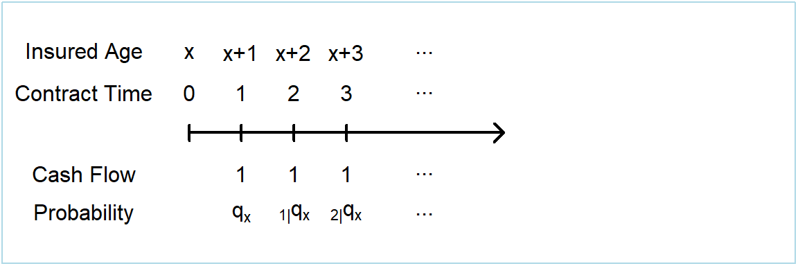
Figure 3.2: Timeline of benefit cash flows from a whole of life insurance policy
We summarize the random variable, mean and variance as follows:
\[ \boxed{ \begin{array}{rcccccc} PV &=& v^{K_{\bf{x}}+1} \\ &=& \sum_{k=0}^{\infty} v^{k+1} ~I(K_{\bf{x}}=k) \\ \mathrm{E}(PV) &=& \sum_{k=0}^{\infty} v^{k+1} ~_{k|}q_{\bf{x}} &=& A_{\bf{x}}\\ \mathrm{Var}(PV) &=& \sum_{k=0}^{\infty} \left( v^{k+1} \right)^2 ~_{k|}q_{\bf{x}} - [\mathrm{E}(PV)]^2 &=& ~^2A_{\bf{x}} - \left( A_{\bf{x}} \right) ^2 .\\ \end{array} } \tag{3.7} \]
This display introduces the actuarial symbols \(A_{\bf{x}}\) and \(^2A_{\bf{x}}\). Here, \(A_{\bf{x}}\) represents the expected present value of the benefits from a whole of life policy on \(\bf{x}\). Similarly, \(^2A_{\bf{x}}\) represents the expected squared present value of the benefits from the same whole of life policy and is used for calculating the variance of the present value. Life insurance actuarial symbols are summarized in Appendix Section 9.1.2.
Example 3.2. Life Insurance by Selected Attributes. To illustrate, consider the Section 2.6 mortality. As a baseline, we consider a healthy female that is not a smoker, not obese, and has an average blood pressure level equal to 114 as well as an interest rate of 4%.
Figure 3.3 summarizes the expected presented values \(A_x\) by age \(x\). The left-hand panel shows expected presented values \(A_x\) by age and gender where the blue solid line represents males and the dark red dashed line represents females. Not surprisingly, values of \(A_x\) vary by age \(x\). Also, for many ages, there are important differences between male and female values. Women tend to enjoy lower mortality rates and so have lower values of \(A_x\).
The right-hand panel gives similar information by smoking status where the blue solid line represents smokers and the dark red dashed line represents nonsmokers. Not surprisingly, smokers have higher mortality and so have higher values of \(A_x\).
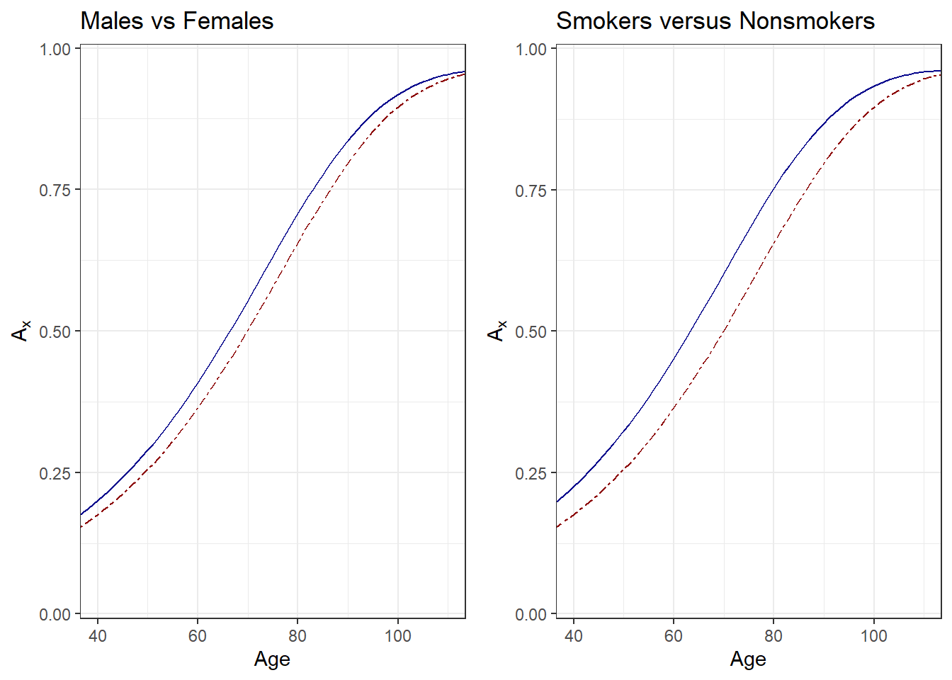
Figure 3.3: Life Insurance by Age, Gender, and Smoking Status. Both panels show expected presented values \(A_x\) by age \(x\). For the left-hand panel, males are shown as solid blue, females as dark red dashed. For the right-hand panel, smokers are shown as solid blue, nonsmokers as dark red dashed.
In the same way, Figure 3.4 shows the relationship between \(A_x\) and \(x\) for different blood pressure levels. Here, blood pressure ranges from 110 (the lowest line) to 170 (the highest line). From the figure, we see that blood pressure becomes increasingly important as \(x\) increases.
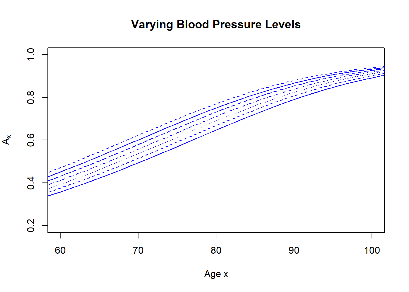
Figure 3.4: Life Insurance by Age and Plood Pressure. A plot of expected presented values \(A_x\) by age \(x\). The lower thick line represents the lowest level of blood pressure, the upper line represents the highest level of blood pressure.
3.2.2 Term insurance
Under a term insurance policy the insurer pays a benefit because of the death of the policyholder within a specified term \(n\) of the policy, with payment made at the end of the year of death. Hence, like whole of life insurance, the payment is made at time \(K_{\bf{x}}+1\), as long as \(K_{\bf{x}}+1\) is less than or equal to the \(n\) year term of the policy. This system is illustrated on a timeline in Figure 3.5, with the \(PV\), \(\mathrm{E}(PV)\) and \(\mathrm{Var}(PV)\) of the benefit cash flows shown in display (3.8). Because the cash flow is contingent on the death of the policyholder, only one payment can be made and hence the calculation of \(\mathrm{Var}(PV)\) from equation (3.4) is valid.
Figure 3.5: Timeline of benefit cash flows from a term insurance policy
\[ \boxed{ \begin{array}{rl} PV &= v^{K_{\bf{x}}+1} I(K_{\bf{x}}+1 \le n) = \left \{\begin{array}{cl} v^{K_{\bf{x}}+1} & \text{where } K_{\bf{x}}+1 \le n \\ 0 & \text{where } K_{\bf{x}}+1 > n \\ \end{array} \right. \\ &= \sum_{k=0}^{n-1} v^{k+1} ~I(K_{\bf{x}}=k) \\ \mathrm{E}(PV) &= \sum_{k=0}^{n-1} v^{k+1} ~_{k|}q_{\bf{x}} = A_{{\bf{x}}:\enclose{actuarial}{n}} ^ {1}\\ \mathrm{Var}(PV) &= \sum_{k=0}^{n-1} \left( v^{k+1} \right)^2 ~_{k|}q_{\bf{x}} - [\mathrm{E}(PV)]^2 = ~^2A_{{\bf{x}}:\enclose{actuarial}{n}} ^ {1} - \left( A_{{\bf{x}}:\enclose{actuarial}{n}} ^ {1} \right)^2 . \\ \end{array} } \tag{3.8} \]
Display (3.8) introduces the actuarial symbols \(A_{{\bf{x}}:\enclose{actuarial}{n}} ^ {1}\) and \(^2A_{{\bf{x}}:\enclose{actuarial}{n}} ^ {1}\). Here, \(A_{{\bf{x}}:\enclose{actuarial}{n}} ^ {1}\) represents the expected present value of the benefits from a term insurance policy on \(\bf{x}\) of term \(n\) years. Similarly, \(^2A_{{\bf{x}}:\enclose{actuarial}{n}} ^ {1}\) represents the expected squared present value of the benefits from the same term insurance policy. It is used for calculating the variance of the present value as per equation (3.2).
Example 3.3. Term Life Insurance. Consider again the baseline case from Example 3.2, a healthy female that is not a smoker, not obese, and has an average blood pressure level equal to 114 as well as an interest rate of 4%.
Figure 3.6 summarizes the expected presented values \(A_{{\bf{x}}:\enclose{actuarial}{n}} ^ {1}\) by age \(x\) and selected values of the term, \(n\). It is not surprising that the effect of term limits diminishes as age increases. Differences among expected present values are most pronounced for the younger ages.
Figure 3.6: Term Life Insurance by Age and Term. A plot of expected presented values \(A_{{\bf{x}}:\enclose{actuarial}{n}} ^ {1}\) by age \(x\) for selected values of the term \(n\).
3.2.3 Pure endowment
Under a pure endowment policy the insurer pays a benefit because of the survival of the policyholder for the \(n\) year term of the policy. In Chapter 2 we defined the random variable \(T_{\bf{x}}\) as being the exact death time (measured in years from the current time) of \(\bf{x}\). The time of the benefit payment is \(n\) but is dependent upon \(T_{\bf{x}}\). This system is illustrated on a timeline in Figure 3.7, with the \(PV\), \(\mathrm{E}(PV)\) and \(\mathrm{Var}(PV)\) of the benefit cash flows shown in display (3.9). Since the cash flow is contingent on the death of the policyholder only one payment can be made and hence the calculation of \(\mathrm{Var}(PV)\) from equation (3.4) is valid.
Figure 3.7: Timeline of benefit cash flows from a pure endowment policy
\[ \boxed{ \begin{array}{rll} PV &= v^n I(T_{\bf{x}}>n) &= \left \{\begin{array}{cl} 0 & \text{where } T_{\bf{x}} \le n \\ v^n & \text{where } T_{\bf{x}} > n \\ \end{array} \right. \\ \mathrm{E}(PV) &= v^n {_np_{\bf{x}}} &= A_{{\bf{x}}:\enclose{actuarial}{n}} ^ {\space \space \space \space \space 1} \\ \mathrm{Var}(PV) &= v^{2n} {_np_{\bf{x}}}(1-{_np_{\bf{x}}}) . \end{array} } \tag{3.9} \]
This display introduces the actuarial symbol \(A_{{\bf{x}}:\enclose{actuarial}{n}} ^ {\space \space \space \space \space 1}\). Here, \(A_{{\bf{x}}:\enclose{actuarial}{n}} ^ {\space \space \space \space \space 1}\) represents the expected present value of the benefits from a pure endowment policy on \(\bf{x}\) of term \(n\) years. Unlike whole of life and term insurance we do not define notation for the expected squared present value of the benefits from the same pure endowment policy as the variance of the present value is simple to express without it, since the \(PV\) is effectively \(v^n\) multiplied by a Bernoulli random variable with parameter \({_np_{\bf{x}}}\).
3.2.4 Endowment insurance
An endowment insurance policy is effectively a combination of a term insurance and pure endowment policy. The insurer pays a benefit at the end of the year of death if the policyholder’s death occurs within the term \(n\) of the policy, or at time \(n\) if the policyholder survives until the term \(n\). This system can be illustrated on a timeline as can be seen in Figure 3.8, with the \(PV\), \(\mathrm{E}(PV)\) and \(\mathrm{Var}(PV)\) of the benefit cash flows shown in display (3.10). Since the cash flow is contingent on the death of the policyholder only one payment can be made and hence the calculation of \(\mathrm{Var}(PV)\) from equation (3.4) is valid.
Figure 3.8: Timeline of benefit cash flows from an endowment insurance policy
\[ \boxed{ {\small \begin{array}{rcccccccc} PV &=& v^{\text {min} \left[ K_{\bf{x}}+1 , n \right]} \ \ \ \ \ \ \ = \left \{\begin{array}{cl} v^{K_{\bf{x}}+1} & \text{where } K_{\bf{x}}+1 \le n \\ v^n & \text{where } K_{\bf{x}}+1 > n \\ \end{array} \right. \\ &=& \sum_{k=0}^{n-1} v^{k+1} ~I(K_{\bf{x}}=k) + v^n ~I(K_{\bf{x}}+1 > n) \\ \mathrm{E}(PV) &=& \sum_{k=0}^{n-1} v^{k+1} ~_{k|}q_{\bf{x}} + v^n ~_np_{\bf{x}} &=& A_{{\bf{x}}:\enclose{actuarial}{n}} = A_{{\bf{x}}:\enclose{actuarial}{n}} ^ {1} + A_{{\bf{x}}:\enclose{actuarial}{n}} ^ {\space \space \space \space \space 1} \\ \mathrm{Var}(PV) &=& \sum_{k=0}^{n-1} \left( v^{k+1} \right)^2 ~_{k|}q_{\bf{x}} + v^{2n} ~_np_{\bf{x}} - [\mathrm{E}(PV)]^2 &=& ~^2A_{{\bf{x}}:\enclose{actuarial}{n}} - \left( A_{{\bf{x}}:\enclose{actuarial}{n}} \right)^2 .\\ \end{array} } } \tag{3.10} \]
This display introduces the actuarial symbols \(A_{{\bf{x}}:\enclose{actuarial}{n}}\) and \(^2A_{{\bf{x}}:\enclose{actuarial}{n}}\). Here, \(A_{{\bf{x}}:\enclose{actuarial}{n}}\) represents the expected present value of the benefits from a endowment insurance policy on \(\bf{x}\) of term \(n\) years. Similarly, \(^2A_{{\bf{x}}:\enclose{actuarial}{n}}\) represents the expected squared present value of the benefits from the same endowment insurance policy and is used for calculating the variance of the present value as per equation (3.2).
3.3 Life Annuity Benefits
In this section, you learn how to:
- Express cash flow indicators for several life annuity benefits including life, term life, deferred life, and guaranteed life contracts.
- Determine moments of each contract and interpret them using traditional actuarial notation in the special case of constant benefits.
- Calculate moments of each contract (using statistical software) and interpret differences due to varying policyholder and contract features.
This section introduces several basic types of life annuity policies. As with Section 3.2, this notation assumes that all cash flows \(_kC\) are \(1\) for simplification. Life annuity actuarial symbols are summarized in Appendix Section 9.1.3.
3.3.1 Life annuity
Under a life annuity policy the insurer pays regular benefits to policyholders whilst they are alive. An annuity payable in advance has benefits paid at the start of the year, while an annuity payable in arrears has benefits paid at the end of the year. This system is illustrated on a timeline in Figure 3.9.
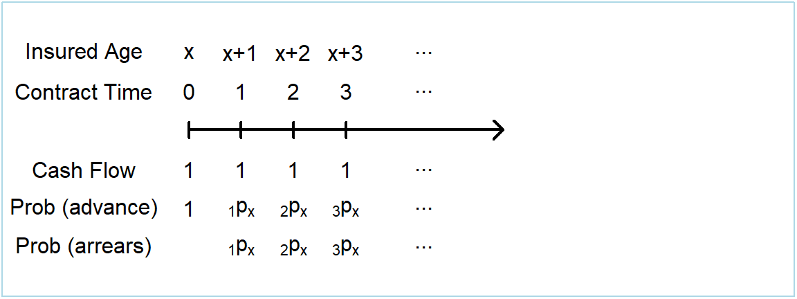
Figure 3.9: Timeline of benefit cash flows from a life annuity policy
The following displays summarize the \(PV\) and \(\mathrm{E}(PV)\) of the benefit cash flows. For payments in advance, we have:
\[ \boxed{ \begin{array}{rl} PV &= 1+v^{1}+v^{2}+ \cdots +v^{K_{\bf{x}}} = \sum_{k=0}^{K_{\bf{x}}} v^k \\ &= \sum_{k=0}^{\infty} v^{k} ~I(K_{\bf{x}} \ge k) \\ \mathrm{E}(PV) &= \sum_{k=0}^{\infty} v^{k} ~_kp_{\bf{x}} = \ddot{a}_{\bf{x}} .\\ \end{array} } \tag{3.11} \]
For payments in arrears, we have:
\[ \boxed{ \begin{array}{rl} PV &= v^{1}+v^{2}+ \cdots +v^{K_{\bf{x}}} \\ &= \sum_{k=0}^{\infty} v^{k+1} ~I(K_{\bf{x}} \ge k+1) \\ \mathrm{E}(PV) &= \sum_{k=0}^{\infty} v^{k+1} ~_{k+1}p_{\bf{x}} = {a}_{\bf{x}} = \ddot{a}_{\bf{x}} - 1 .\\ \end{array} } \tag{3.12} \]
These displays introduce the actuarial symbols \(\ddot{a}_{\bf{x}}\) and \({a}_{\bf{x}}\). Here, \(\ddot{a}_{\bf{x}}\) and \({a}_{\bf{x}}\) represent the expected present value of the benefits from a life annuity policy on \(\bf{x}\), in advance and in arrears respectively. The variance of present values can be calculated using the general expression in equation (3.6) with, in this special case, \(~_kIC\) \(=v^{2k}+ 2v^{k} \ddot{a}_{\enclose{actuarial}{k}}\).
A special case of interest occurs when the yield curve is flat so that \(_ki=i\). Then, the \(PV\) in equations (3.9) and (3.10) above can also be expressed using actuarial notation from financial mathematics. For example, for a life annuity in advance:
\[ PV =1+v^{1}+v^{2}+\cdots +v^{K_{\bf{x}}} \space = \ddot{a}_{\enclose{actuarial}{K_{\bf{x}}+1}} = \frac{1+i}{i} \left( 1-v^{K_{\bf{x}}+1} \right) . \tag{3.13} \]
Remember that the present value of benefits from a whole of life policy is equal to \(v^{K_{\bf{x}}+1}\). Therefore this relationship can be used to examine a relationship between life annuities and whole of life policies, starting from the \(PV\) of a life annuity in advance as follows:
\[ \boxed{ \begin{array}{rcccccccc} PV &=& \frac{1+i}{i} \left( 1-v^{K_{\bf{x}}+1} \right) \\ \mathrm{E}(PV) &=& \mathrm{E} \left[ \frac{1+i}{i} \left(1-v^{K_{\bf{x}}+1} \right) \right] &=& \frac{1+i}{i} \left(1- \mathrm{E} \left[ v^{K_{\bf{x}}+1} \right] \right) \\ \ddot{a}_{\bf{x}} &=& \frac{1+i}{i} \left(1- A_{\bf{x}} \right) \\ \mathrm{Var}(PV) &=& \mathrm{Var} \left[ \frac{1+i}{i} \left(1-v^{K_{\bf{x}}+1} \right) \right] \\ &=& \left( \frac{1+i}{i} \right) ^2 \mathrm{Var} \left[ v^{K_{\bf{x}}+1} \right] &=& \left( \frac{1+i}{i} \right) ^2 \left( ~^2A_{\bf{x}} - \left( A_{\bf{x}} \right) ^2 \right) . \end{array} } \tag{3.14} \]
The relationships in equations (3.13) and (3.14) hold only when \(_ki = i\), but do provide an intuitive calculation of the variance of the present value of a life annuity. However, the restrictive assumption of a flat yield curve makes this relationship less useful in practice and so we will not consider it in further detail.
Example 3.4. Life Annuities by Age, Interest Rate, and Gender. To illustrate, we return to the insurance mortality used in Example 3.2. Figure 3.10 summarizes the expected presented values \(\ddot{a}_x\) by age, interest rate, and gender. As with insurances, for many ages, there are important differences between male and female values. Because women tend to enjoy lower mortality rates, they have higher values of \(\ddot{a}_x\). Not surprisingly, values of \(\ddot{a}_x\) vary by age \(x\) and interest rate \(i\). The figure emphasizes that the interest rate produces greater differences in \(\ddot{a}_x\) for younger ages than older ages.
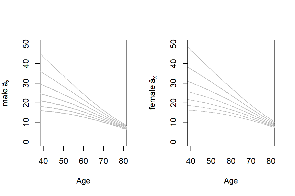
Figure 3.10: Life Annuities by Age, Interest Rate, and Gender. Male annuities are in the left-hand panel, those for females are in the right. For both panels, each line corresponds to an interest rates with the top line being \(i=0\) and the bottom line being \(i=0.06\).
Figure 3.10a. Interactive Version of Figure 3.10. Use the mouse to rotate the figure to see different perspectives. One can use this plot to motivate a type of multiplicative effect that an interest rate and age has on an annuity value.
3.3.2 Term life annuity
Under a term life annuity policy the insurer pays benefits to policyholders whilst they are alive, for a maximum of \(n\) periods. For annuities in advance and in arrears, this system is illustrated on a timeline in Figure 3.11, with the \(PV\) and \(\mathrm{E}(PV)\) of the benefit cash flows shown in displays (3.15) and (3.16).

Figure 3.11: Timeline of benefit cash flows from a term life annuity policy
In advance:
\[ \boxed{ \begin{array}{rl} PV &= 1+v^{1}+v^{2}+ \cdots +v^{\text{min}[K_{\bf{x}},n-1]} \\ &= \sum_{k=0}^{n-1} v^{k} ~I(K_{\bf{x}} \ge k) \\ \mathrm{E}(PV) &= \sum_{k=0}^{n-1} v^k ~_kp_{\bf{x}} = \ddot{a}_{{\bf{x}}:\enclose{actuarial}{n}} .\\ \end{array} } \tag{3.15} \]
In arrears:
\[ \boxed{ \begin{array}{rl} PV &= v^{1}+v^{2}+ \cdots +v^{\text{min}[K_{\bf{x}},n]} \\ &= \sum_{k=0}^{n-1} v^{k+1} ~I(K_{\bf{x}} \ge k+1) \\ \mathrm{E}(PV) &= \sum_{k=0}^{n-1} v^{k+1} ~_{k+1}p_{\bf{x}} = {a}_{{\bf{x}}:\enclose{actuarial}{n}} .\\ \end{array} } \tag{3.16} \]
These displays introduce the actuarial symbols \(\ddot{a}_{{\bf{x}}:\enclose{actuarial}{n}}\) and \({a}_{{\bf{x}}:\enclose{actuarial}{n}}\). Here, \(\ddot{a}_{{\bf{x}}:\enclose{actuarial}{n}}\) and \({a}_{{\bf{x}}:\enclose{actuarial}{n}}\) represent the expected present value of the benefits from a term life annuity policy on \(\bf{x}\), in advance and in arrears respectively. The variance of present values can be calculated using the general expressions in equations (3.5) and (3.6).
3.3.3 Deferred life annuity
Under a deferred life annuity policy the insurer pays benefits to policyholders whilst they are alive, but only after a deferral period of \(n\) periods. For annuities in advance and in arrears, this system is illustrated on a timeline in Figure 3.12, with the \(PV\) and \(\mathrm{E}(PV)\) of the benefit cash flows shown in displays (3.17) and (3.18).
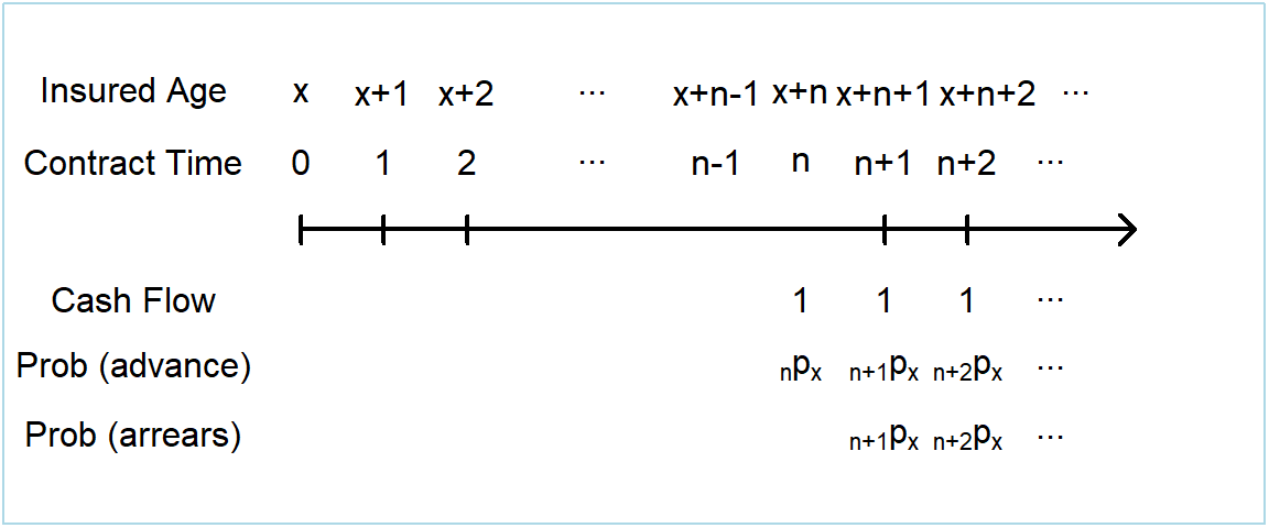
Figure 3.12: Timeline of benefit cash flows from a deferred life annuity policy
In advance:
\[ \boxed{ \begin{array}{rl} PV &= \left \{\begin{array}{cl} 0 & \text{where } T_{\bf{x}} < n \\ v^{n}+v^{n+1}+v^{n+2}+ \cdots +v^{K_{\bf{x}}} & \text{where } T_{\bf{x}} \ge n \\ \end{array} \right. \\ &= \sum_{k=n}^{\infty} v^{k} ~I(K_{\bf{x}} \ge k) \\ \mathrm{E}(PV) &= \sum_{k=n}^{\infty} v^k ~_kp_{\bf{x}} = ~_{n|}\ddot{a}_{\bf{x}} = \ddot{a}_{\bf{x}} - \ddot{a}_{{\bf{x}}:\enclose{actuarial}{n}} .\\ \end{array} } \tag{3.17} \]
In arrears:
\[ \boxed{ \begin{array}{rl} PV &= \left \{\begin{array}{cl} 0 & \text{where } T_{\bf{x}} < n+1 \\ v^{n+1}+v^{n+2}+ \cdots +v^{K_{\bf{x}}} & \text{where } T_{\bf{x}} \ge n+1 \\ \end{array} \right. \\ &= \sum_{k=n}^{\infty} v^{k+1} ~I(K_{\bf{x}} \ge k+1) \\ \mathrm{E}(PV) &= \sum_{k=n}^{\infty} v^{k+1} ~_{k+1}p_{\bf{x}} = ~_{n|}{a}_{\bf{x}} = {a}_{\bf{x}} - {a}_{{\bf{x}}:\enclose{actuarial}{n}} .\\ \end{array} } \tag{3.18} \] These displays introduce the actuarial symbols \(_{n|}\ddot{a}_{\bf{x}}\) and \(_{n|}{a}_{\bf{x}}\). Here, \(_{n|}\ddot{a}_{\bf{x}}\) and \(_{n|}{a}_{\bf{x}}\) represent the expected present value of the benefits from a deferred life annuity policy on \(\bf{x}\), in advance and in arrears respectively.
3.3.4 Guaranteed life annuity
A guaranteed life annuity policy is the same as a life annuity policy, except that the benefits are guaranteed to be paid for a minimum of \(n\) periods. For annuities in advance and in arrears, this system is illustrated on a timeline in Figure 3.13, with the \(PV\) and \(\mathrm{E}(PV)\) of the benefit cash flows shown in displays (3.19) and (3.20).
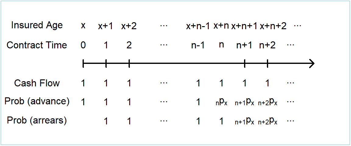
Figure 3.13: Timeline of benefit cash flows from a guaranteed life annuity policy
In advance:
\[ \boxed{ \begin{array}{rl} PV &= 1+v^{1}+v^{2}+ \cdots +v^{\text{max}[K_{\bf{x}},n-1]} \\ &= \sum_{k=0}^{n-1} v^{k} + \sum_{k=n}^{\infty} v^{k} ~I(K_{\bf{x}} \ge k) \\ \mathrm{E}(PV) &= \sum_{k=0}^{n-1} v^k + \sum_{k=n}^{\infty} v^k ~_kp_{\bf{x}} = \ddot{a}_{\overline{{\bf{x}}:\enclose{actuarial}{n}}} = \ddot{a}_{\enclose{actuarial}{n}} + ~_{n|}\ddot{a}_{\bf{x}} .\\ \end{array} } \tag{3.19} \]
In arrears:
\[ \boxed{ \begin{array}{rl} PV &= v^{1}+v^{2}+ \cdots +v^{\text{max}[K_{\bf{x}},n]} \\ &= \sum_{k=0}^{n-1} v^{k+1} + \sum_{k=n}^{\infty} v^{k+1} ~I(K_{\bf{x}} \ge k+1) \\ \mathrm{E}(PV) &= \sum_{k=0}^{n-1} v^{k+1} + \sum_{k=n}^{\infty} v^{k+1} ~_{k+1}p_{\bf{x}} = {a}_{\overline{{\bf{x}}:\enclose{actuarial}{n}}} = {a}_{\enclose{actuarial}{n}} + ~_{n|}{a}_{\bf{x}} .\\ \end{array} } \tag{3.20} \]
These displays introduce the actuarial symbols \(\ddot{a}_{\overline{{\bf{x}}:\enclose{actuarial}{n}}}\) and \({a}_{\overline{{\bf{x}}:\enclose{actuarial}{n}}}\). Here, \(\ddot{a}_{\overline{{\bf{x}}:\enclose{actuarial}{n}}}\) and \({a}_{\overline{{\bf{x}}:\enclose{actuarial}{n}}}\) represent the expected present value of the benefits from a deferred life annuity policy on \(\bf{x}\), in advance and in arrears respectively.
3.4 Valuing Life Contingent Benefits using a Spreadsheet
In this section, you learn how to:
- Calculate moments of life insurance and life annuity contracts using spreadsheet methods.
Traditional approaches to valuing life insurances and life annuities, presented in Sections 3.2 and 3.3 respectively, emphasize constant cash amounts (taken to be one without loss of generality) and constant rates of interest. Although important, there are also many instances where cash benefits and interest rates vary over time. An advantage of a spreadsheet or a flexible programming approach is that there are no important restrictions on the cash flows nor interest rates, as long as they are known in advance.
The structure presented in Section 3.1 readily accommodates these extensions. So, to see how they might work in practice, in this section we show the important calculations using a spreadsheet approach. That is, the calculations are performed in a spreadsheet in such a way to allow flexibility to adjust age (\(x\)), term (\(n\)), cash flows (\(_kC\)), interest rates (\(_ki\)) and life table mortality rates (\(q_x\)). Display 3.2 shows a workbook that can be viewed and downloaded.
Display 3.2. Spreadsheet Calculations of Life Contingent Benefits
There are three tabs in the Display 3.2 worksheet. Initially appearing is the third tab called Assum & Outp - var C that contains calculations and results, allowing for a variable \(_kC\). The calculations are performed using the first principles of equations (3.2), (3.3) and (3.4). Cells highlighted in yellow can be changed to adjust \(x\), \(n\), \(_kC\) and \(_ki\). Cells highlighted in orange provide the output calculations for the benefits described in Section 3.2. Similar timing conventions are adopted to that of the previous worksheet, with the cash flows occurring at the beginning (\(k\)) or end (\(k+1\)) of the year.
The first tab, denoted as Life Table, contains yellow highlighted \(q_x\) cells can be adjusted as desired.
The second tab, denoted as Assum & Outp - fixed C, contains calculations and results, assuming that \(_kC\) equals a fixed \(C\). This allows the use of the notation introduced in Section 3.2. Cells highlighted in yellow can be changed to adjust \(x\), \(n\), \(C\) and \(_ki\). Cells highlighted in orange provide the output calculations for the benefits described in Section 3.2. In this and the next worksheet a column “Year” is introduced which is equal to \(k+1\). The column is introduced so that we may think of the cash flows as related to a profit year for an insurer, which we will introduce in Chapter X. Various calculation columns for both \(k\) and \(k+1\) are calculated, to account for cash flows occurring at the beginning of the year (e.g. life annuities in advance) and cash flows occurring at the end of a year (e.g. life annuities in arrears) whilst still allocating these cash flows to the same year.
You are recommended to review the formulae in the workbook against those found in Section 3.1 and 3.2, to confirm your understanding of how to perform the calculations in a spreadsheet package. The calculations are not performed in R, although a case study using R will be provided in Section 3.5.
3.5 Case Study: A Portfolio of Term Insurance Policies
In this section, you learn how to:
- Determine the distribution of the present value of an insurance contract using statistical software.
- Summarize the moments of a portfolio of contracts.
- Determine the distribution of a portfolio of contracts, using simulation as well as a normal approximation.
Now let us consider a collection, or portfolio, of several contracts. For simplicity, we assume that all contracts are of the term insurance type introduced in Section 3.2.2. We do allow contract policyholders to have different ages and gender as well as choosing different contract terms and amounts insured. For notation, we use the subscript \(j\) to differentiate among contracts and so denote individual features as \({\bf{x}}_j\) where \(j = 1,2, \ldots,J\) using \(J\) for the number of contracts.
We constructed a portfolio that mimics others that we have seen in practice. We assume that policyholders from the final year of the insurer data (i.e. Month 780) purchase a term insurance policy, giving us \(J=190\). The policyholder data can be obtained by clicking on this link. For illustrative purposes, we assume that mortality follows that described in Example 3.2. For these data, it turns out that there 136 females and 54 males in the portfolio. Figure 3.14 summarizes the distributions of initial ages, contract terms, and sums insured.
R Code to Summarize Policyholder Information from the Portfolio
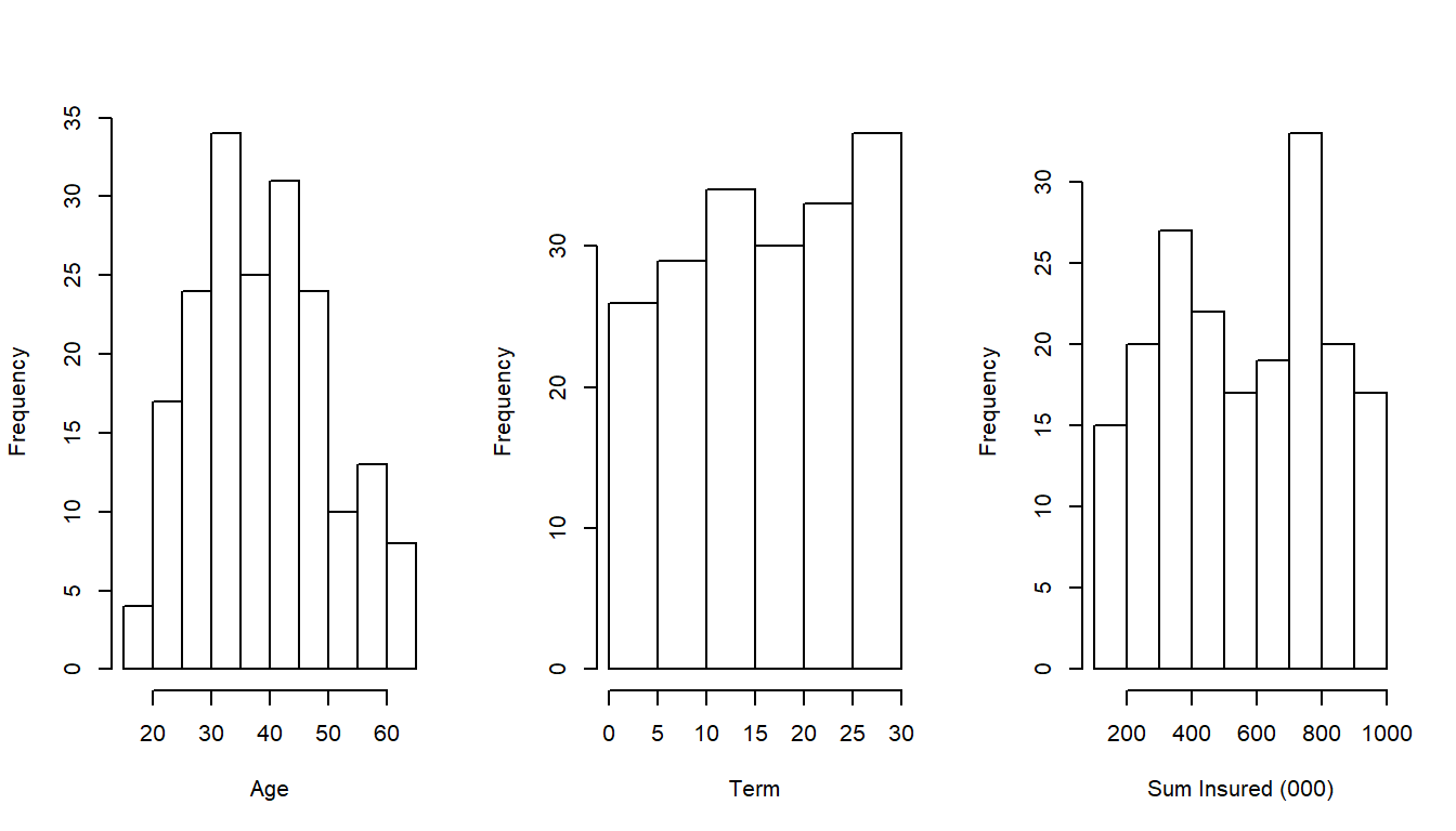
Figure 3.14: Portfolio Characteristics
3.5.1 An individual policy
To see how valuation of these uncertain cash flows work, we start by examining a single policy from the portfolio. Specifically, we consider a healthy female aged \(x=50\) at the purchase of the policy with mortality described in Example 3.3. To demonstrate the flexibility of these methods, unlike this example, for discounting we use the spot rates specified in Display 3.2. Further we assume this individual has purchased a term insurance policy with term \(n=10\) years with a sum insured of $400,000 (\(=~_kC\)) and that we wish to value the policy immediately after purchase.
As we did in Section 3.4, we can begin the valuation calculations of \(\mathrm{E}(PV)\) and \(\mathrm{Var}(PV)\), based on the results from display (3.8), using a spreadsheet.
Display 3.3. Valuation of an individual policy
Display 3.3 summarizes the results where we see that the expected present value for this policy is 13,981. The display also shows the variance and, after taking a square root, we see that the standard deviation is 67,637. As we will learn in Chapter 5, expected present values are good approximations for a policy premium and so are easy to interpret. In contrast, it is difficult to interpret the standard deviation for a single contract. However, single contract standard deviations are important ingredients that are used to build variances and standard deviations for portfolios that are meaningful quantities.
The following R code can be used to perform the same calculations as in Display 3.3.
R Code For Term Insurance Individual Example
Distribution of Present Values. Another way of analysing the random present value \(PV\) is to investigate its distribution. From display (3.8), we see that \(PV\) is a function of the random \(K_{\bf{x}}\), a discrete random variable. Thus, \(PV\) is also discrete. We can use knowledge of the probability mass function (pmf) of \(K_{\bf{x}}\), \(\Pr(K_{\bf{x}}=k) = ~_{k|}q_{\bf{x}}\), to determine the pmf of \(PV\).
In this example we denote \(~_kPV = 400,000v^{k+1}\) for \(k \in \{0,1,2,3,\ldots,9\}\) and \(~_kPV = 0\) otherwise. Therefore the probability mass function of \(PV\) is \(\Pr \left( PV= ~_kPV \right) = ~_{k|}q_{49}\) where \(k \in \{0,1,2,3,\ldots,9\}\) and \(\Pr \left( PV= 0 \right) = ~_{10}p_{49}\). These values are:
R Code for pmf calculation
| kPV | 392157 | 384468 | 376929 | 369538 | 362292 | 355189 | 348224 | 341396 | 334702 | 328139 | 0 |
| Pr(PV = kPV) | 0.0024 | 0.0026 | 0.003 | 0.0033 | 0.0037 | 0.0042 | 0.0047 | 0.0052 | 0.0058 | 0.0065 | 0.9586 |
Note the large proportion of the distribution at \(PV=0\) (over 95% for this example). This is common in life insurance applications. Among other things, this means that the distribution is not even approximately normal and so specialized techniques are required to summarize the distribution. Nonetheless, as we see in the following subsections, the distribution of a portfolio of policies may well be approximately normally distributed.
3.5.2 Moments of a portfolio of policies
We now return to the portfolio of \(J=190\) policies. Using display (3.8), the present value for the \(j\)th policy is
\[ PV_j = v^{K_{{\bf{x}}_j}+1} I(K_{{\bf{x}}_j}+1 \le n_j) . \] Using display (3.8) and incorporating the variable sum insured \(C_j\) and term \(n_j\), for this portfolio we can describe the present value, its expectation, and variance as:
\[ \boxed{ \begin{array}{rl} PV &= \sum_{j=1}^J PV_j \\ \mathrm{E}(PV) &= \sum_{j=1}^J \mathrm{E}(PV_j) = \sum_{j=1}^J C_j \left \{\sum_{k=0}^{n_j-1} v^{k+1} ~_k|q_{{\bf{x}}_j} \right\} \\ &= \sum_{j=1}^J C_j ~ A_{{\bf{x}_j}:\enclose{actuarial}{n_j}} ^ {1} \\ \mathrm{Var}(PV) &= \sum_{j=1}^J \left\{\mathrm{E}(PV_j^2) - [\mathrm{E}(PV_j)]^2 \right\} \\ &= \sum_{j=1}^J C_j^2 \left\{ ~ ~^2A_{{\bf{x}_j}:\enclose{actuarial}{n_j}} ^ {1} - [ ~ A_{{\bf{x}_j}:\enclose{actuarial}{n_j}} ^ {1} ]^2 \right\}.\\ \end{array} } \tag{3.21} \]
We can calculate the portfolio mean and standard deviation using display (3.21). It turns out that the expected portfolio value is 5516 and the standard deviation is 1290, both in thousands of dollars. This is done in the following R code.
R Code For Term Insurance Portfolio Example EPV
3.5.3 Simulated distribution of a portfolio of policies
The mean and variance are useful summary measures but we would really like to know the entire distribution of potential outcomes for the portfolio. In many actuarial applications, it is common to encounter situations far too complex to analyze analytically. Typically, in actuarial practice one turns to simulation of results. For one introduction to simulation, see the chapter in the open textbook Loss Data Analytics on Simulation and Resampling.
For this portfolio, even if the insured policyholders are independent across all \(j\), determining the exact distribution of \(PV\) is typically not possible. Instead we use simulation to gain a greater understanding of the distribution of \(PV\). The following code shows the output of 500 simulated observations of \(PV\) from equation (3.21), including the mean, standard deviation and a histogram.
R Code For Term Insurance Portfolio Example Simulations
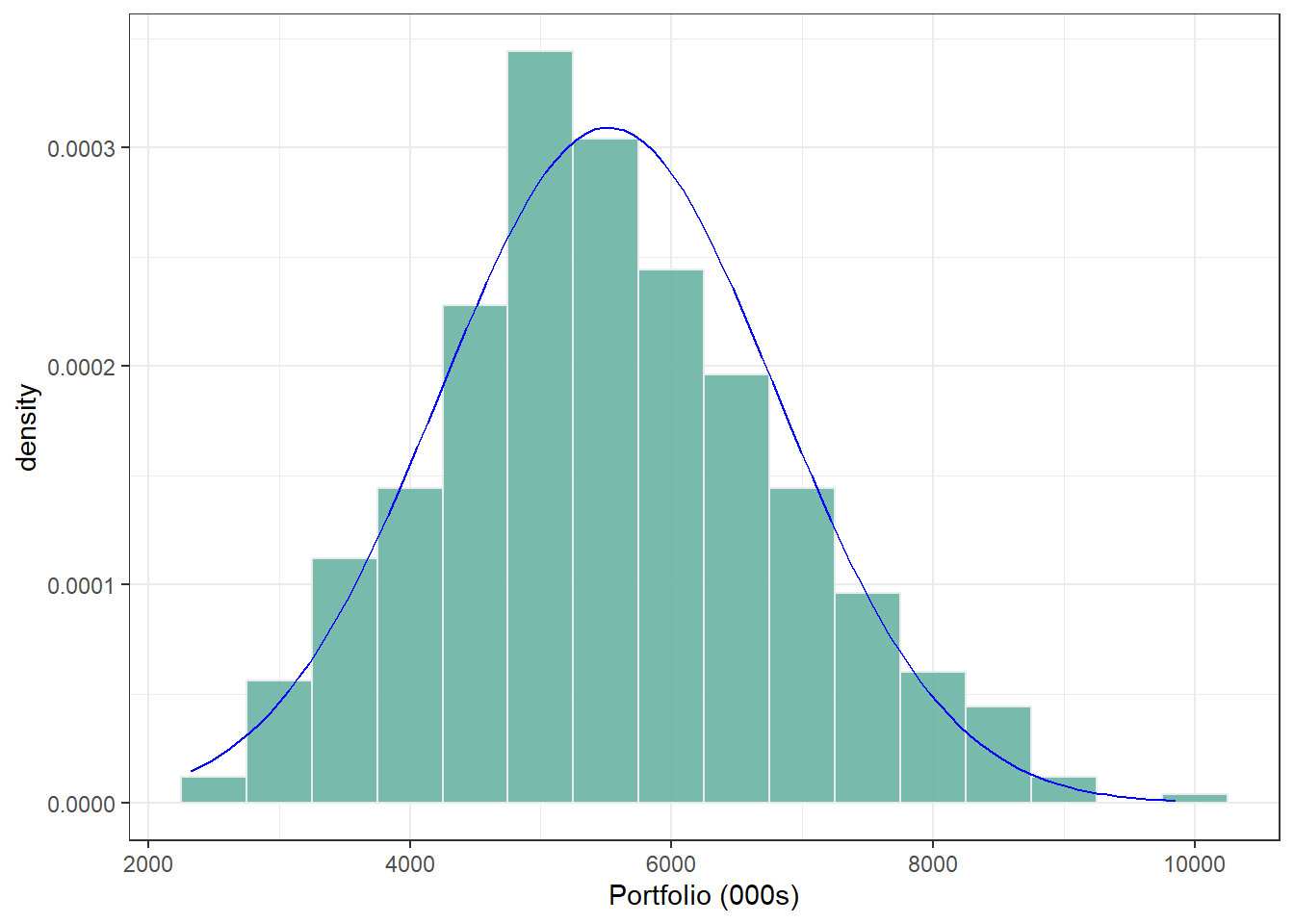
Figure 3.15: Distribution of \(PV\) for a portfolio of policyholders
Two things are immediately apparent from the simulated observations of \(PV\) from the portfolio of policies.
- Despite the extreme skewness of the \(PV\) outcomes for an individual policyholder, the distribution of the \(PV\) of the portfolio of policies is remarkably bell shaped. This is evidence of the Central Limit Theorem in action.
- Whilst the standard deviation of the \(PV\) of an individual policy is many times larger than the \(E(PV)\), the standard deviation of the \(PV\) of a portfolio of policies is multiple times smaller than the \(E(PV)\).
From both of the observations, we learn that the standard deviation (and variance) is helpful in understanding the uncertainty of a portfolio. This is despite our observation in the case of a single policy where we saw that the standard deviation was not helpful because of the large mass at zero of the distribution. We will revisit this point again in later chapters when investigating the financial condition of a life insurer.
3.6 Further Resources and Contributors
Contributors
- Adam Butt, Australian National University, and Edward (Jed) Frees, University of Wisconsin-Madison & Australian National University, are the principal authors of the initial version of this chapter. Email: jfrees@bus.wisc.edu for chapter comments and suggested improvements.