Chapter 6 Empirical Exercises
\(\require{enclose}\)
6.1 Chapter 2 Empirical Exercises
Exercise 2.3.1. Gompertz-Makeham and Survival Probabilities. Recall the U.S. Life Expectancies introduced in Section 2.1:
| Age | Total | Male | Female | Hispanic..Total | Hispanic..Male | Hispanic..Female |
|---|---|---|---|---|---|---|
| 0 | 78.6 | 76.1 | 81.1 | 81.8 | 79.1 | 84.3 |
| 20 | 59.4 | 57.0 | 61.8 | 62.5 | 59.9 | 64.9 |
| 40 | 40.7 | 38.7 | 42.6 | 43.5 | 41.2 | 45.5 |
| 60 | 23.3 | 21.7 | 24.7 | 25.5 | 23.6 | 27.0 |
| 80 | 9.2 | 8.4 | 9.8 | 10.5 | 9.4 | 11.1 |
Section 2.3 used these data to fit a Gompertz-Makeham distribution for female lives; in this exercise, we repeat this analysis but for male lives. To this end,
- Fit a Gompertz-Makeham model to the provided US Male life expectancies.
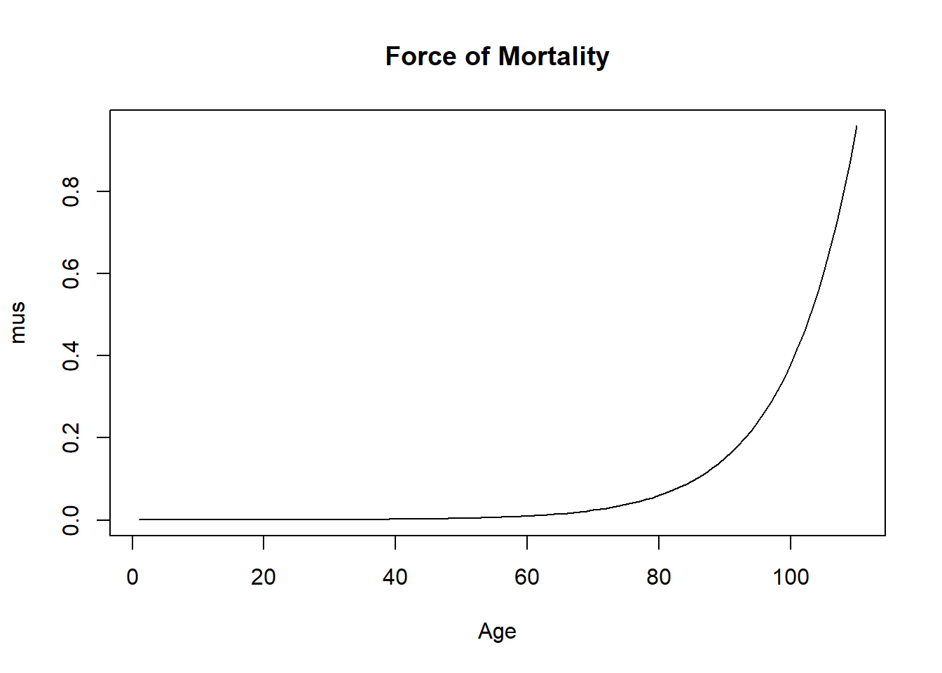
- Plot the resulting force of mortality and the survival function, compare to the one for U.S. Females from Section 2.3.
- Determine the resulting model to determine the probabilities that a 20 year old survives to age 60, 70, and 80: \(~_{40}p_{20}\), \(~_{50}p_{20}\), and \(~_{60}p_{20}\).
Exercise 2.3.1 Solution
Exercise 2.4.1. Creating a Life Table from One-Year Central Decrements. In this exercise, we will create a life table based on one-year central decrements using data from the Human Mortality Database.
- Download the data from Appendix Section 8.1. Create a subset of the data for year 2015 using female rates.
- From these central death rates, create one-year mortality rates.
- Starting with 100,000 lives at age 0, create a life table. Use \(\omega=111\) as the limiting age. List the first six rows of your table.
Exercise 2.4.1 Solution
6.2 Chapter 3 Empirical Exercises
Exercise 3.2.1. Whole Life Actuarial Present Values.
In Exercise 2.4.1, we learned how to create a life table based on one-year central decrements using data from the Human Mortality Database. In this exercise, we use this life table to explore life insurance calculations in R. We first include columns for \(A_x\) – the actuarial present values for whole life insurance – and the corresponding second moment. We then use this information to determine term and endowment insurances.
The following code demonstrates how this works for females lifes. Then, you are asked to replicate this analysis for male lives.
Add Columns for \(A_x\) and \(^2A_x\)
Starting with the life table you created in Exercise 2.4.1, next you will add columns for \(A_x\) and \(^2A_x\). For that, we need to fix the interest rate. Given currently low rates, we choose \(i=2\%\).
We then determine \(A_x\) and \(^2A_x\) via their recursion relationships, where we start with \(\omega = 111\) for which \(A_{\omega}=v\) and \(^2A_{\omega}=v^2\):
R Code to Determine Whole Life Actuarial Present Values
Here is an excerpt from our now more complete life table:
     Year_start Age       mx        qx      l      Ax   TwoAx
1817       2015  40 0.001388 0.0013870 975424 0.43823 0.20726
1818       2015  41 0.001470 0.0014689 974071 0.44622 0.21454
1819       2015  42 0.001621 0.0016197 972640 0.45435 0.22207
1820       2015  43 0.001736 0.0017345 971065 0.46256 0.22979
1821       2015  44 0.001861 0.0018593 969381 0.47090 0.23775
1822       2015  45 0.002044 0.0020419 967578 0.47935 0.24596
Term and Endowment Insurance
Let’s use it for pricing life insurance contracts. Let’s set \(x=40\) and \(n=20\), and evaluate pure endowment, term life, and endowment insurance:
R Code to Determine Whole Life Actuarial Present Values
Let’s also calculate corresponding standard deviations (square roots of variances):
R Code to Determine Standard Deviations
Repeat the above calculations above for the US male population. To this end, you should:
- complete the male life table with columns for \(A_x\) and \(^2A_x\);
- determine pure endowment, term life, and endowment insurance values and standard deviations for a forty year old male and a 20 year term; and
R Code to Determine Whole Life Actuarial Present Values
Exercise 3.2.2. Increasing Insurance Actuarial Present Values. As a follow-up to Exercise 3.2.1, we now consider an increasing whole life insurance. To begin, we determine the present value of an increasing insurance policy, using the basic summation, \[ (IA)_x = \sum_{k=0}^{\omega} {_kp_x}\,q_{x+k}\,v^{k+1}\,(k+1). \] Here it is:
R Code to Determine APV Increasing Whole Life
Alternatively, we can evaluate the increasing insurance present value as the sum of deferred insurance contracts:
\[ (IA)_x = \sum_{k=0}^{\omega} {_{k|}A_x}. \]
Carrying it out…
R Code APV of Increasing Whole Life based on Deferred Contracts
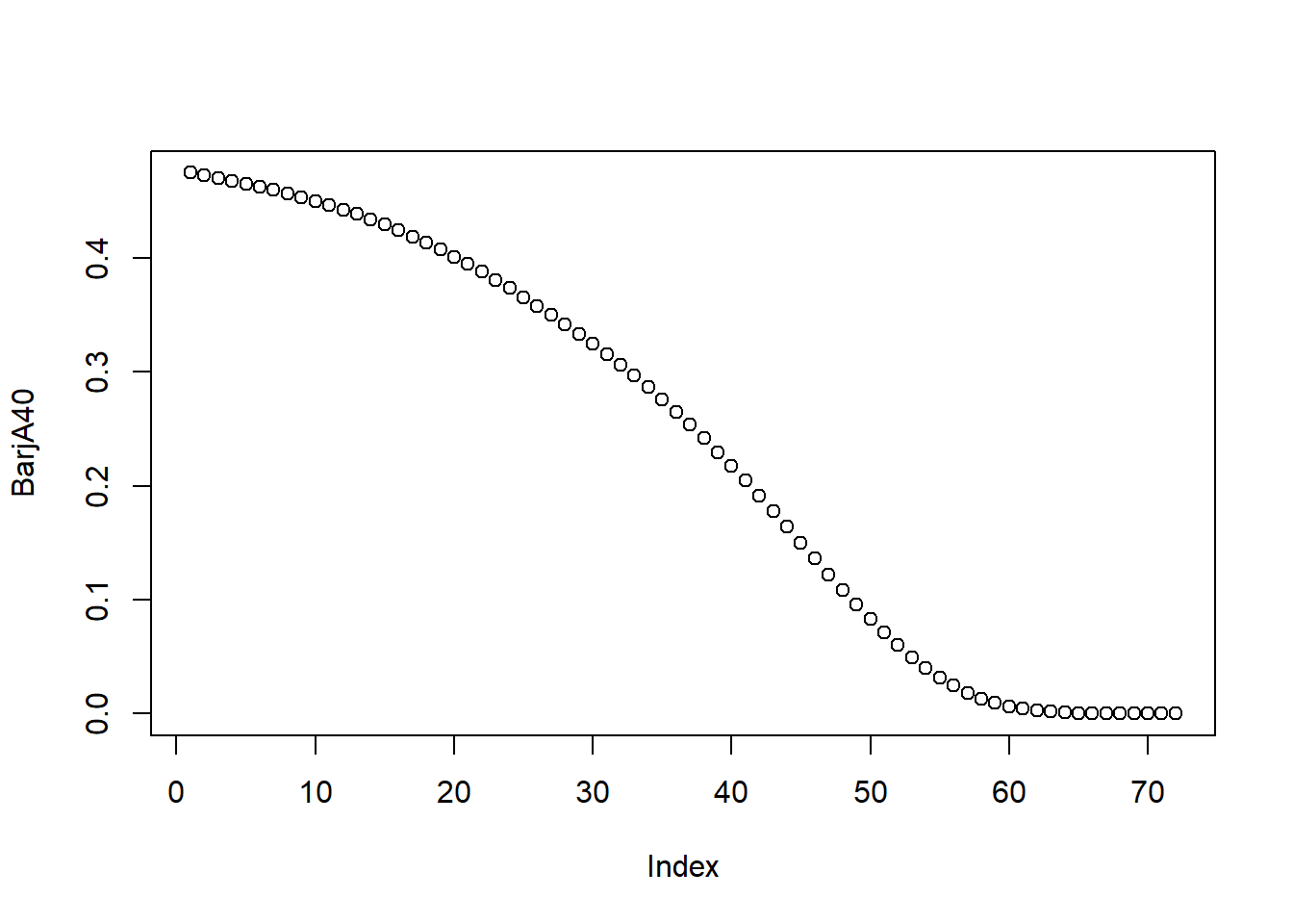
We can also plot the deferred insurance actuarial present values:
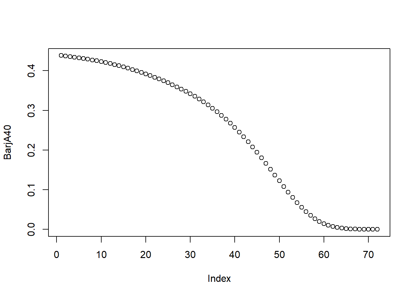
Let’s also evaluate the second moment, which we obtain by squaring the payoff and the discount factors:
R Code for Second Moments of Increasing Whole Life
We can use it to determine the standard deviation:
[1] 2.41Repeat the above calculations above for the US male population. Specifically, for an increasing whole life insurance on a 40-year old male insured, you should determine the
- actuarial present value and
- the associated standard deviation
R Code to Determine Whole Life Actuarial Present Values
6.3 Chapter 4 Empirical Exercises
Section 4.3 Exercises
Exercise 4.3.1. Actuarial Present Values for Select and Ultimate Tables. The select and ultimate tables introduced in Section 4.3.2 are complicated – is such complexity is warranted in practice? To get insights into this question, in this exercise you will compare actuarial present values derived from select and ultimate mortality to those from only ultimate mortality. To be specific, we focus consider whole life insurance for using the female Canadian experience introduced in Section 4.3.2; the data are available in Appendix Section 8.4.
For these data,
- produce \(A_x\) for \(x=50, \ldots, 65\) using an interest rate of \(i=0.04\) based on
- select and ultimate mortality
- ultimate mortality
- compare these two sequences of actuarial present values by calculating their ratio.
- repeat parts (a) and (b) using an interest rate \(i=0.02\).
To give you a feel for the results, Figure 6.1 summarizes the results.
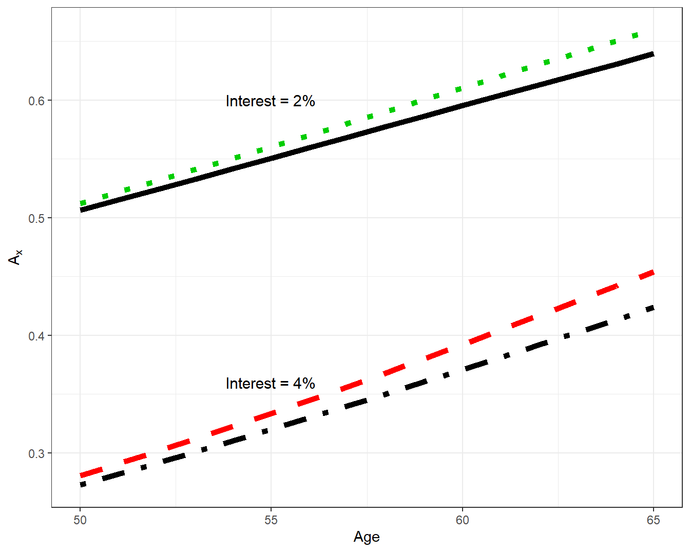
Figure 6.1: Life Insurance APV by Age, Interest, and Mortality Type. A plot of life insurance actuarial present value \(A_x\) by age \(x\). The top two lines are based on \(i=0.02\), the bottom two based on \(i=0.04\). For each pair, the top line uses ultimate mortality, the bottom line is based on select and ultimate mortality
Exercise 4.3.1 Answer
Section 4.5 Exercises
Exercise 4.5.1. Dog Survival Distributions and Actuarial Present Values. The analysis in Section 4.5.2 suggests that breed is an important factor for dog survival. To underscore this point for a broader audience, let us look at survival for a type of small dog, a “Jack Russell Terrier”, and a large dog, a “German Shepherd Dog”. We can make differences in survival distributions between small and large dogs even more meaningful by also computing selected actuarial present values that summarize future expected costs.
You should begin your analysis by downloading the data, available in Appendix Section 8.3.
The data have been re-worked so that they can be used for your analysis. Here is a bit more code needed to convert data fields appropriately and to separate the file into two subsets, one for Terriers and one for German Shepherds.
Show R Code to Pre-Process the Data
For these data:
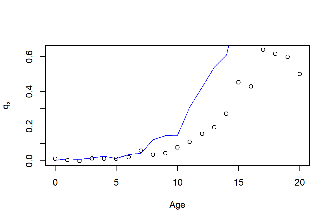
- Compute one-year mortality rates for both Terriers and German Shepherds. Do this over \(x=0, \ldots, 20\). Graph the results.
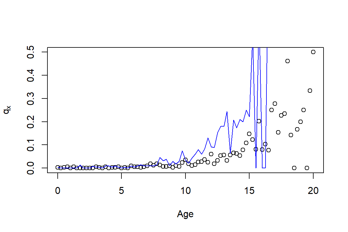
- Because you may be working with products with events occurring more frequently than once a year, you decide to follow the strategy introduced in Section 4.1.1 and look at mortality rates occurring on a quarterly basis. Repeat the analysis from part (a) using quarterly rates.
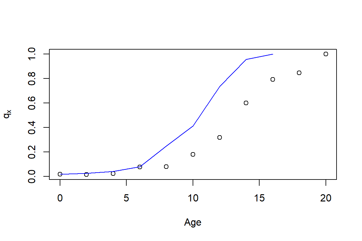
- The results of earlier analyses indicate substantial volatility in the both quarterly rates and annual rates at later ages. One approach to mitigate this volatility is to smooth the rates. A simpler approach is to use longer periods (hence increasing exposure and reducing volatility). Repeat the analysis in part (a) using rates on a once every two year basis.
- To see how these rates might be used, you decide to repeat the analysis in Section 4.5.3 and compute an actuarial present value of the lifetime cost of surgical vet care. Use the same assumptions as in that section with the initial annual cost as 458, \(i=0.03\) interest rate and a 11 percent annual growth in surgical care costs. However, use the dog mortality from part (a). Do this for \(x=2, 5, 12\), for both breeds. You will see that that your results on German Shepherds differ slightly from those presented in Section 4.5.3; comment on why this is so.