Chapter 2 Modeling Lifetimes

The analysis of life contingent exposures such as insurer’s liability when selling a life insurance contract or a pension fund’s obligations when offering a new pension scheme starts with modeling individual lifetime and death. These models, in turn, have to be calibrated in the context of relevant (mortality) data.

Therefore, in this chapter, we first present different types of data that describe the lifetimes and mortality of a certain population. We deliberately introduce the data in Section 2.1 without assuming prior knowledge of life contingent modeling, and aim to develop an intuitive understanding of some of the associated challenges.

We then introduce the conventional framework for modeling lifetimes, particularly by introducing the concept of a future lifetime variable \(T_{\bf x}\) and its properties, and we then explore various approaches of specifying and estimating its distribution. Here, we discuss the traditional actuarial models for lifetimes such as analytical mortality laws and life tables, but we also introduce conditional predictive models that characterize the lifetime distribution based on a set of covariates or features.

2.1 Mortality data: Life Expectancies, Deaths, Counts, & Lifetimes

2.1.1 Life Expectancies

Perhaps the most relevant question to any individual when it comes to their future lifetime is: how long am I expected to live? As we will discuss, there are many angles to this question. However, as a first and proximate answer, we may rely on public statistics. Government agencies around the world publish vital statistics such as the life expectancies for their population, which are typically separated by age and gender – and potentially other attributes such as race.

The file CDCLifeExp.csv is provided with the supplemental information of this text and includes an excerpt of the U.S. national vital statistics that provides “Expectation of life, by age, race, […] and sex: United States, 2017” in Table 2.1.

library(knitr)
us_les <- read.csv("Data/CDCLifeExp.csv")
kable(us_les, caption="Life Expectancies From 2017 U.S. National Vital Statistics")

Table 2.1: Life Expectancies From 2017 U.S. National Vital Statistics

Age	Total	Male	Female	Hispanic..Total	Hispanic..Male	Hispanic..Female
0	78.6	76.1	81.1	81.8	79.1	84.3
20	59.4	57.0	61.8	62.5	59.9	64.9
40	40.7	38.7	42.6	43.5	41.2	45.5
60	23.3	21.7	24.7	25.5	23.6	27.0
80	9.2	8.4	9.8	10.5	9.4	11.1

This excerpt provides the life expectancy for ages 0 (newborn), 20, 40, 60, and 80 observed within a population, for males and females with separate figures for the hispanic subpopulation. There are a few immediate observations.

First, females generally seem to have a longer life expectancy than males, whereas the aggregate “Total” life expectancy is in between the two figures. This is intuitive as the aggregate population is (largely) made up of male and female individuals, so that the “Total” life expectancy is a weighted average of the gender-specific life expectancies, relative to the composition of the population.

Second, life expectancy is decreasing in age, which again is intuitive: older individuals will have shorter life expectancies, ceteris paribus. It may be somewhat less obvious that the differences in life expectancies are less than the differences in age; subtracting the lines in Table 2.1 gives incremental life expectancies for 20-year age gaps.

kable(us_les[1:4,2:7]-us_les[2:5,2:7])

Total	Male	Female	Hispanic..Total	Hispanic..Male	Hispanic..Female
19.2	19.1	19.3	19.3	19.2	19.4
18.7	18.3	19.2	19.0	18.7	19.4
17.4	17.0	17.9	18.0	17.6	18.5
14.1	13.3	14.9	15.0	14.2	15.9

Hence, while a 40-year-old male is twenty years older than a 20-year-old male, the 20-year-old’s life expectancy is 18.3 years higher. The difference of 1.7 years is due to the possibility of the 20-year-old not surviving up to age 40. Consider the following: 40-year-old males lived 20 years since age 20 plus they are expected to live another 38.7 years, for a total of 58.7 years; in contrast, 20-year-old males have a life expectancy of 57 years, which is 1.7 years less. In other words, 40-year-old males have a higher expected age at death than 20-year-old males, because we view them conditionally on already having lived until age 40. As the table reveals, this effect is more pronounced when comparing a 40-year-old with a 60-year-old or a 60-year-old with an 80-year-old.

Third, the life expectancies for the hispanic sub-population exceed the figures of the total population, which suggests that other subpopulations must exhibit a lower life expectancy. There are many questions of potential reasons for this difference, although these fall more in the demographic or even sociological realm. For instance, there are many interesting studies related to the dependence of life expectancies on socio-economic factors, including some concerning recent trends related to so-called “deaths of despair” in the U.S.

From an actuarial perspective, a relevant question may be how we could model the mortality data. In other words, is there a simple parametric model that may describe the progression of life expectancy across ages, at least in the context of one particular population? We will return to this question in the context of our mortality models, particularly in Section 2.3.

As an early caveat to the question raised at the beginning of this section, it is not necessarily accurate to take these figures as estimates of a given individual’s future lifetime or even its expectation. This is the case since the life expectancy is usually generated based on recent mortality experience rather than forecasts. As we will discuss in Section 2.4, this is the difference between the so-called period and cohort life expectancies.

2.1.2 Population Mortality Counts

We now bring into consideration mortality experience for populations that had been observed over time, which is available at the Human Mortality Database (HMD) for a wide range of countries. The available data include Exposures by age, sex, and calender year period, i.e. how many people of a given age and sex lived in the country’s population during a given period of time, and corresponding Deaths, i.e. how many of these individuals had died.

In the supplemental information to this text, we provide exposures and deaths for the U.S. population, downloaded from the HMD as HMD_Expo.csv and HMD_Deaths.csv. We use the data over five year intervals starting at 1935 until 2015. Let us take a look at the exposures:

us_exp <- read.csv("Data/HMD_Expo.csv")

kable(head(us_exp), align = "cccrrr", digits = 2, format.args = list(big.mark = ","))

Year_start	Year_end	Age	Female	Male	Total
1935	1939	0	4,869,267	5,057,569	9,926,836
1935	1939	1	4,802,597	4,936,238	9,738,835
1935	1939	2	5,119,574	5,244,634	10,364,208
1935	1939	3	5,159,494	5,287,402	10,446,896
1935	1939	4	5,189,350	5,307,754	10,497,104
1935	1939	5	5,359,159	5,531,967	10,891,126

and deaths:

us_deaths <- read.csv("Data/HMD_Deaths.csv")

kable(head(us_deaths), align = "cccrrr", digits = 2, format.args = list(big.mark = ","))

Year_start	Year_end	Age	Female	Male	Total
1935	1939	0	253,145.89	335,492.00	588,637.89
1935	1939	1	36,010.02	42,169.20	78,179.22
1935	1939	2	17,718.83	21,208.22	38,927.05
1935	1939	3	12,450.36	14,852.17	27,302.53
1935	1939	4	10,154.85	11,771.25	21,926.10
1935	1939	5	8,678.43	10,339.57	19,018.00

To illustrate, let us plot the exposures and deaths for a 70-year-old U.S. females over time, which is given in Figure 2.1:

R Code For Figure

options(digits = 9)
options(scipen = 9)
par(mfrow=c(1,2))
plot(us_exp[us_exp$Age == 70,2], us_exp[us_exp$Age == 70,4]/1000, type = "l", lwd = 5, col = "green", main="Exposures", xlab = "year", ylab = "count", ylim = c(0,max(us_exp[us_exp$Age == 70,4])/1000))
plot(us_deaths[us_deaths$Age == 70,2], us_deaths[us_deaths$Age == 70,4]/1000, type = "l", lwd = 5, col = "red", main="Deaths", xlab = "year", ylab = "count", ylim = c(0,max(us_deaths[us_deaths$Age == 70,4])/1000))

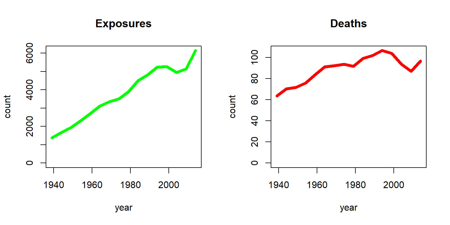
Figure 2.1: Exposures and Deaths (in thousands) for Females age 70 from the HMD U.S.

The stark increase in exposures is due to two effects; on one hand, the U.S. population had been growing substantially since 1935, and on the other hand, individuals had been showing an enhanced life expectancy over time. As a consequence, the number of 70-year-old U.S. females had increased from less than two million to more than six million. In contrast, the number of deaths had been more steady. While with an increasing number of exposures the number of deaths have increased, the chance of dying for a 70-year-old had been decreasing. The latter becomes more evident by plotting the ratio of deaths and exposures as in Figure 2.2.

R Code For Figure

par(mfrow=c(1,1))
minlim <- min(us_deaths[us_deaths$Age == 70,4]/us_exp[us_exp$Age == 70,4])
maxlim <- max(us_deaths[us_deaths$Age == 70,4]/us_exp[us_exp$Age == 70,4])
plot(us_deaths[us_deaths$Age == 70,2],us_deaths[us_deaths$Age == 70,4]/us_exp[us_exp$Age == 70,4],type = "l", lwd = 5, col = "blue", main="Deaths/Exposures", xlab = "year", ylab = "rate",ylim = c(minlim,maxlim))
rm(minlim, maxlim)

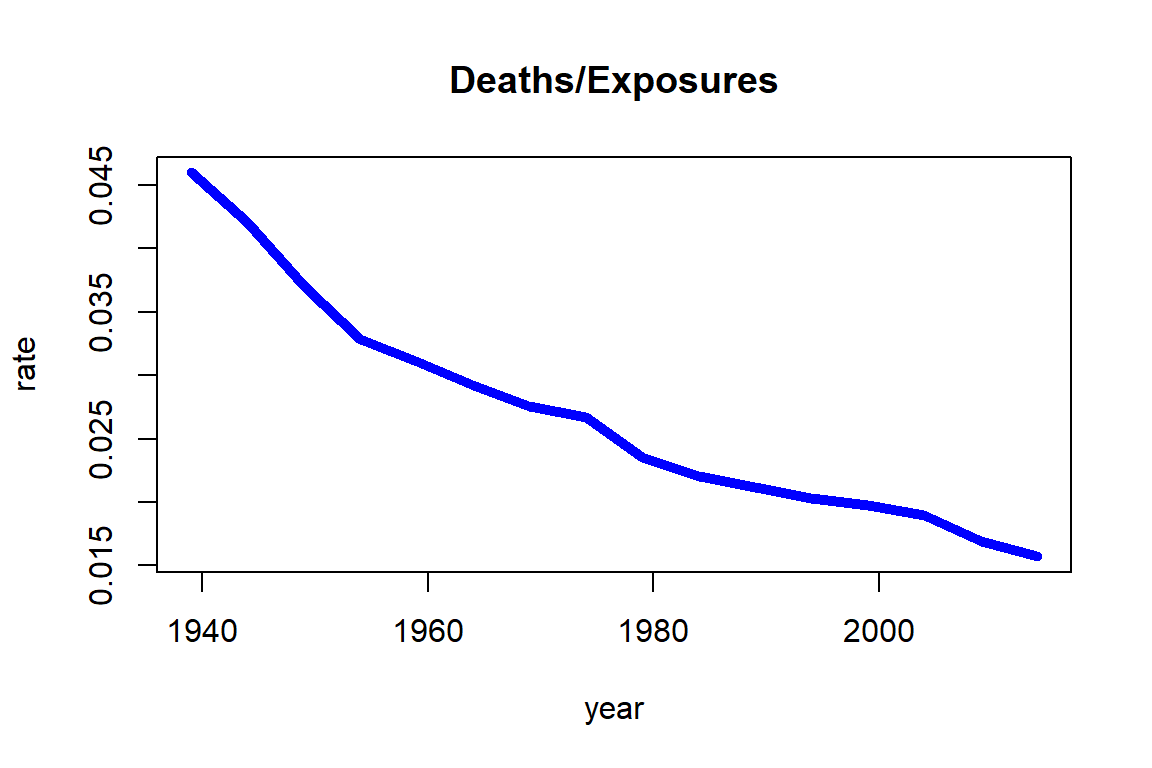
Figure 2.2: Death rates for Females age 70 from the HMD U.S

Note that the chance of dying for a 70-year-old female was more than 4% around 1940, but it had decreased over time to a level lower than 2%. As we will see in Section 2.4, the ratio of deaths and exposures is closely related to death rates.

Alternatively, we can focus on a specific period – say the most recent five years in our data, i.e. 2010-2014 – and plot the deaths over exposures across ages as in Figure 2.3.

R Code For Figure

us_mx_fem_2014 <- us_deaths[us_deaths$Year_start == 2010,4]/us_exp[us_exp$Year_start == 2010,4]
us_mx_mal_2014 <- us_deaths[us_deaths$Year_start == 2010,5]/us_exp[us_exp$Year_start == 2010,5]
plot(us_mx_fem_2014,type = "l", lwd = 5, col = "blue", main="Deaths/Exposures", xlab = "year", ylab = "death rate", ylim = c(min(us_mx_fem_2014),max(us_mx_fem_2014)))

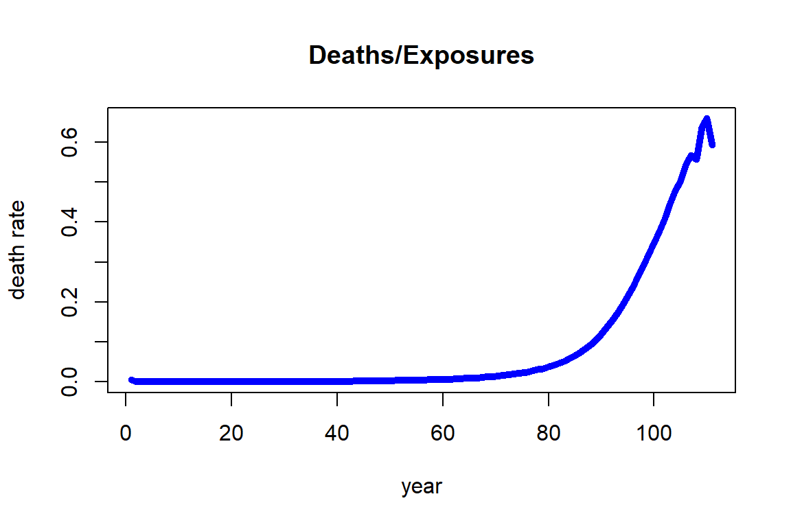
Figure 2.3: Death rates for Females across ages for 2010-2014 from the HMD U.S.

We observe that the death rate increases fairly regularly with respect to age and its growth looks exponential. This observation is the foundation for the most famous and common analytic mortality model that is detailed in Section 2.3 known as the Gompertz law. It should be noted that the death rates at higher ages, specifically from 106 to 110, are showing a larger variability. The reason for this observation is that the number of people alive at those ages (exposures) is relatively small, so that the estimates are more uncertain than those at lower ages.

We note some precaution when using the Human Mortality Database (HMD). It is intended to provide a wide range of interested parties with detailed and up-to-date mortality and population data covering about 41 countries. There are some countries that may exhibit different mortality patterns from these 41 countries, and these include some of the most populous countries such as China, India, and Indonesia, and several countries in the African continent such as South Africa, Nigeria, and Egypt.

2.1.3 Individual Mortality Data

While mortality counts are a common way to organize mortality data across a large population, which had been our emphasis in the previous section, the individual survival time data may provide valuable pieces of information. Indeed, the data available to an insurance company typically consists of records of individuals. The company records individual details for each insured person from when they purchased the contract; these include personal characteristics such as sex, age, date-of-birth, etc., but also medical records and other underwriting information. In addition, the company knows whether or not the person had died at the current time—and, if so, the time of death.

This latter aspect is common for survival or event history data. For each observation (individual) \(i\), we are given a number of covariates or features \(\textbf{x}_i\), as well as the event time \(T_i\) if the event has already happened. Otherwise, we only know that by the current cutoff time, the event has not happened yet. In the context of survival analysis, which is the branch of statistics that deals with survival or event data, this is known as (right) censoring, i.e. the data are (right-)censored.

Data protection policies are omnipresent and insurance companies are not any different with respect to policyholder data. On one hand, there are data protection regulations that disallow disclosure of personal identifiable pieces of information. On the other hand, data are a key resource to a life insurer and sharing this valuable piece of information may create a disadvantage by revealing important information to the company’s competitive position. Therefore, rather than relying on real survival data, we consider a synthetic dataset consisting of a hypothetical portfolio of policyholders.

In the supplemental information to this text, we provide survival information for a hypothetical insurance company in SyntheticInsurerData.csv. The company has sold whole life insurance policies, i.e. policies that pay a death benefit upon the policyholder’s death, since 1955 (the coming chapters discuss different life insurance policies in detail). Policyholders have to go through an underwriting examination, and in addition to policyholders’ age, sex (0 for female, 1 for male), smoking status (0 for non-smoker, 1 for smoker), and the month of sale, the company records the applicants body-mass index (BMI) and the systolic blood pressure at the time of underwriting. Finally, for those policyholders with a claim, i.e., for the policyholders that have died, the company records the time of death (relative to the month of underwriting). The data is organized in the order of sales, so that the oldest entries are at the top of the data and the newest entries are at the bottom:

library(data.table)
ins_data <- fread("Data/SyntheticInsurerData.csv",data.table=FALSE)
kable(head(ins_data), align = "ccccrrrr",digits = 2)
#displaying the very end of the table similar to the very top of the table requires a few more steps
tmp_tail_ins_data <- tail(ins_data); rownames(tmp_tail_ins_data) <- NULL
kable(tmp_tail_ins_data, align = "ccccrrrr",digits = 2)

Month_of_Sale	Age	Sex	Smoking	BMI	BloodPressure	Claim	Time_of_death
1	27	0	0	25.8	117	YES	55.63
1	51	1	0	17.6	109	YES	18.53
1	59	1	0	22.5	132	YES	15.88
1	37	1	0	22.9	109	YES	57.40
1	62	0	0	30.9	147	YES	27.83
1	31	0	0	17.3	91	YES	64.06

Month_of_Sale	Age	Sex	Smoking	BMI	BloodPressure	Claim	Time_of_death
780	43	0	0	17.10	110	NO	NA
780	57	1	1	19.30	118	NO	NA
780	40	0	0	20.10	117	NO	NA
780	27	1	0	20.60	90	NO	NA
780	55	1	1	20.10	118	NO	NA
780	23	1	0	19.03	82	NO	NA

Evidently, most of the policies sold in the first months—back in 1955—have matured, and most recently underwritten policyholders are still alive.

Let us further investigate the mortality data. We start by summarizing the attributes of our data:

suppressWarnings(library(psych))
tmp_describe_ins_data<-psych::describe(ins_data)
kable(tmp_describe_ins_data, digits = 2, format.args = list(big.mark = ","))

	vars	n	mean	sd	median	trimmed	mad	min	max	range	skew	kurtosis	se
Month_of_Sale	1	160,781	394.58	216.72	382.00	393.08	277.25	1.0	780.0	779.0	0.08	-1.17	0.54
Age	2	160,781	39.99	11.61	39.00	39.65	11.86	19.0	65.0	46.0	0.22	-0.73	0.03
Sex	3	160,781	0.70	0.46	1.00	0.75	0.00	0.0	1.0	1.0	-0.87	-1.25	0.00
Smoking	4	160,781	0.30	0.46	0.00	0.25	0.00	0.0	1.0	1.0	0.88	-1.22	0.00
BMI	5	160,781	22.79	4.55	21.70	22.20	3.85	16.1	69.6	53.5	1.46	3.26	0.01
BloodPressure	6	160,781	114.74	15.75	114.00	114.36	16.31	57.0	208.0	151.0	0.26	0.09	0.04
Claim*	7	160,781	1.37	0.48	1.00	1.34	0.00	1.0	2.0	1.0	0.54	-1.71	0.00
Time_of_death	8	59,382	28.27	13.69	28.36	28.24	15.21	0.0	64.2	64.2	0.02	-0.73	0.06

In summary, there are 160,781 insureds, out of which 59,382, i.e. 36.93%, have died; the average age at purchase is about 40, and our portfolio has a high percentage of men (70%) and non-smokers (70%). The average BMI is 22.8 and the average blood pressure is 114.7, which are close to (but somewhat lower than) U.S. national averages; for details on common BMI and blood pressure levels, see e.g. the Withings Health Observatory that provides real-time information for U.S. Americans.

To illustrate the sales history, we plot the monthly sales of the company, which is given as Figure 2.4.

R Code For Figure

monthly_sales <- rep(0,780)
for (i in 1:780){
  monthly_sales[i] <- sum(ins_data$Month_of_Sale == i)
}
plot(monthly_sales,type = "l", lwd = 2, col = "green", main="Monthly Sales", xlab = "month", ylab = "Sales")
abline(h = mean(monthly_sales), col = "red", lty = 2)

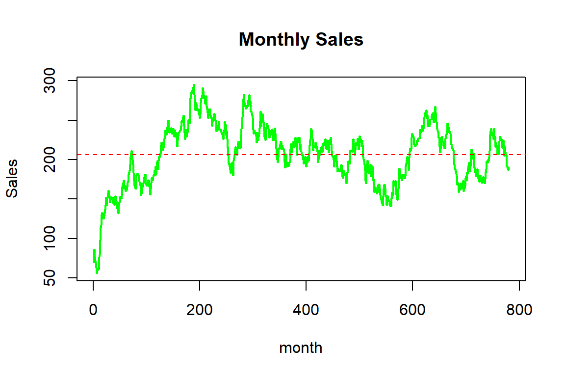
Figure 2.4: Monthy sales for the synthetic mortality data

In summary, the company sells about 200 insurance contracts each month, although there is some variation over time; while sales initially increased, the company experienced some ebbs and flows, potentially due to marketing efforts and/or the effectiveness or attractiveness of the products.

We now investigate the traits of the insureds for which various histograms are given as Figure 2.5.

R Code For Figure

par(mfrow=c(1,3))
hist(ins_data$Age,main="Insured Age", xlab="age", border="red", col="green")
hist(ins_data$BMI,main="Body Mass Index", xlab="bmi", border="red", col="green")
hist(ins_data$BloodPressure,main="Systolic Blood Pressure", xlab="bp", border="red", col="green")

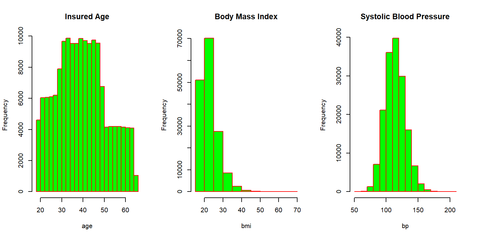
Figure 2.5: Histograms for the synthetic mortality data

Most individuals are in between thirty and fifty years of age when purchasing the coverage, but some sales to younger and some older individuals are observed. The Body Mass Index (BMI) is concentrated between 20 and 30, although there are some outliers with relatively large values. The systolic blood pressure is roughly bell shaped, with most applicants exhibiting blood pressure measurements at normal levels (below 120) or slightly elevated levels (120-130). We further visualize the relationship between these three attributes by looking at the correlation matrix corresponding to these three characteristics, which is given as Figure 2.6.

R Code For Figure

suppressWarnings(library(corrplot))
tmp_corr_ins_data <- cor(ins_data[,c(2,5,6)])
colnames(tmp_corr_ins_data) <- c("Age", "BMI", "BP")
rownames(tmp_corr_ins_data) <- c("Age", "BMI", "BP")
corrplot(tmp_corr_ins_data, method="circle", order="hclust", addCoef.col = "red", tl.col="black",tl.srt=45)

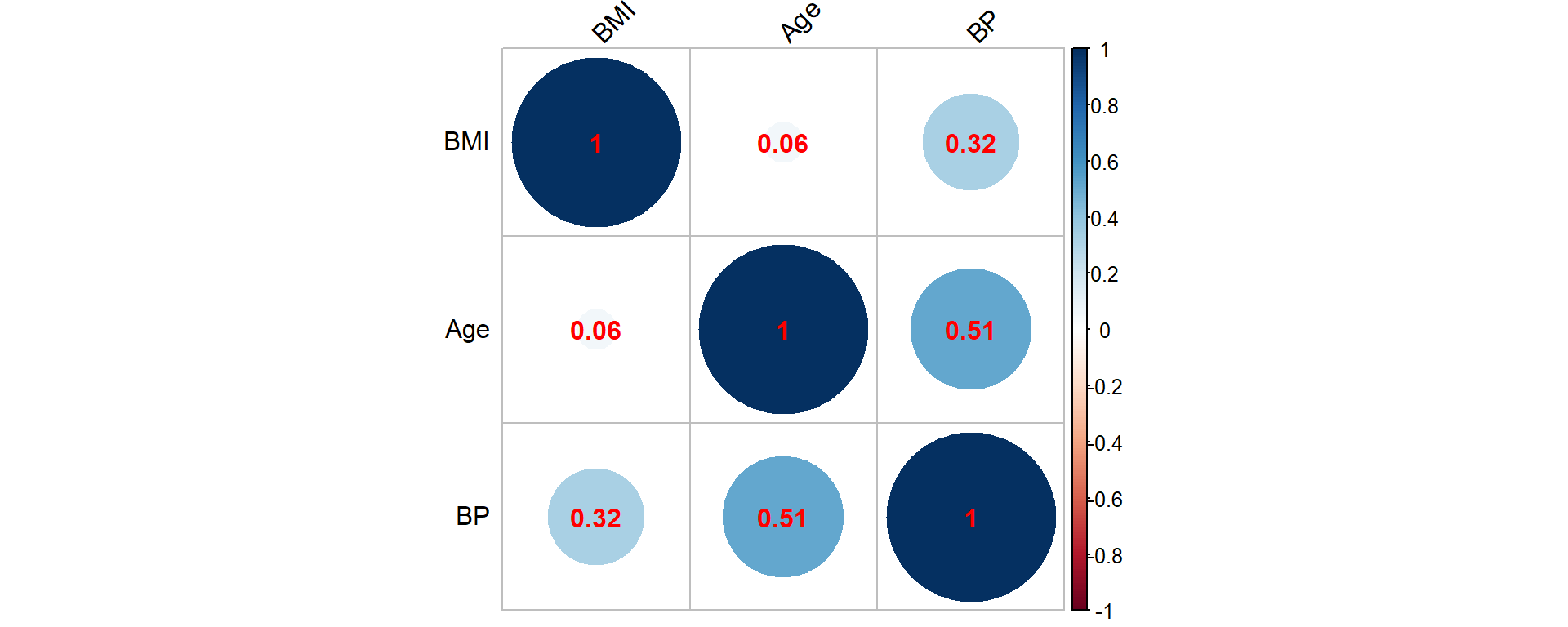
Figure 2.6: Correlation matrix for the synthetic mortality data corresponding to age, BMI and BP (blood pressure)

Clearly, high blood pressure and elevated BMI are positively associated, and an elevated blood pressure is more common for elderly insureds. These are common observations in many populations.

One of our main areas of focus is the realized lifetime, which can only be observed for those individuals where a claim had been paid. We thus plot the distribution of the age at death based on these observations, which is illustrated in Figure 2.7.

hist(ins_data$Age+ins_data$Time_of_death,main="Age at Death", xlab="age", border="red", col="green")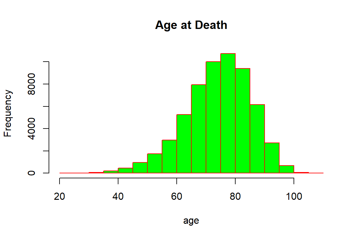

Figure 2.7: Age at Death for the synthetic mortality data

Not surprisingly, the majority of deceased policyholders have died at higher ages: the bulk of deaths are concentrated between seventy and ninety years of age. There are a few individuals that died relatively young, and similarly a few that were close to achieving the centenarian status, though it should be noted that some policyholders at higher ages may still be alive. Indeed, the ages of the five oldest individuals that are still alive are:

round(tail(sort(ins_data[ins_data$Claim=="NO",2]+(780-ins_data[ins_data$Claim=="NO",1])/12),5),digits=2)

[1] 102.50 102.67 103.50 104.17 105.58

It is intuitive that the number of deaths are associated with sales: The maximal number of deaths is the number of individuals that purchased insurance. This is evident when plotting the number of deaths by the year of sale, which is displayed in Figure 2.8, particularly over the early years.

R Code For Figure

annual_death <- rep(0,65)
for (i in 1:65){
  for (j in 1:12){
    annual_death[i] <- annual_death[i] + sum(ins_data[ins_data$Month_of_Sale == (i-1)*12 +j,7] == "YES") 
  }
}
plot(annual_death,type = "l", lwd = 4, col = "blue", main="Annual Deaths", xlab = "Year", ylab = "Deaths")

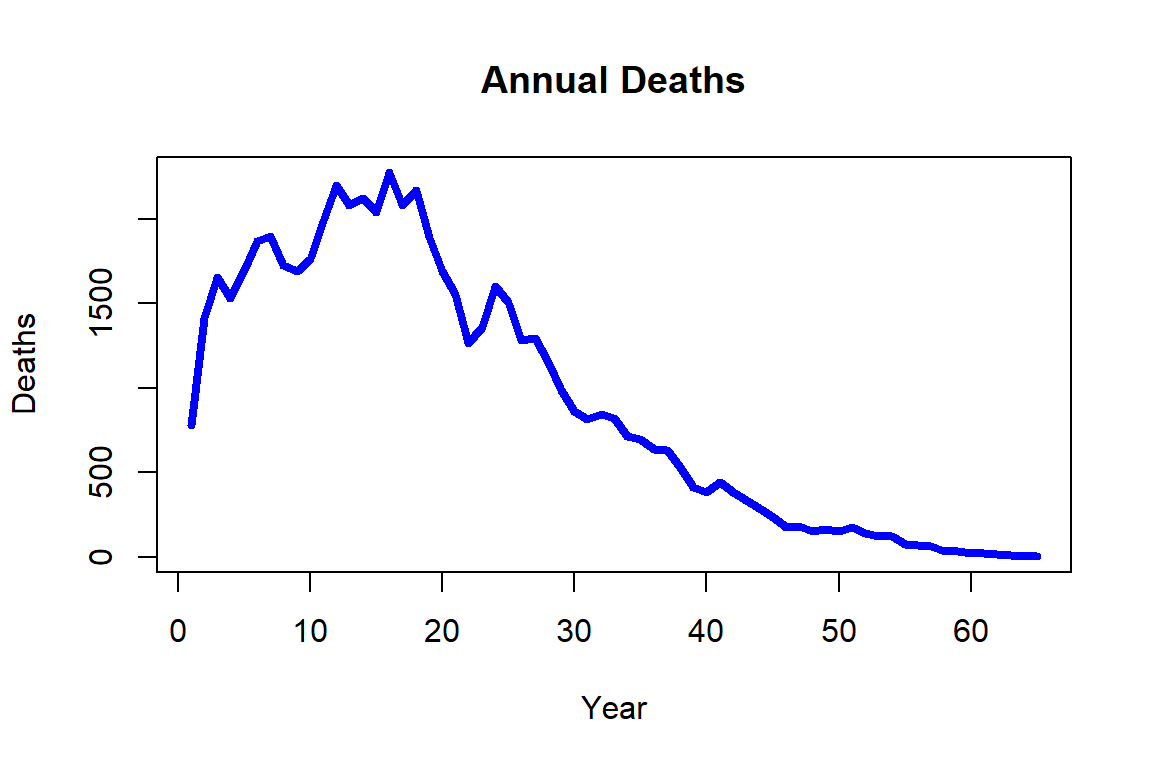
Figure 2.8: Annual deaths for the synthetic mortality data

We can also investigate the relationship of the time of death to policyholder characteristics by creating a correlation plot amongst those that had already died. The correlation matrix appears as Figure 2.9.

R Code For Figure

#suppressWarnings(library(corrplot))
tmp_dead_corr_ins_data <- cor(ins_data[ins_data$Claim == "YES",c(2,5,6,8)])
colnames(tmp_dead_corr_ins_data) <- c("Age", "BMI", "BP", "TD")
rownames(tmp_dead_corr_ins_data) <- c("Age", "BMI", "BP", "TD")
corrplot(tmp_dead_corr_ins_data, method="circle", order="hclust", addCoef.col = "red", tl.col="black", tl.srt=45)

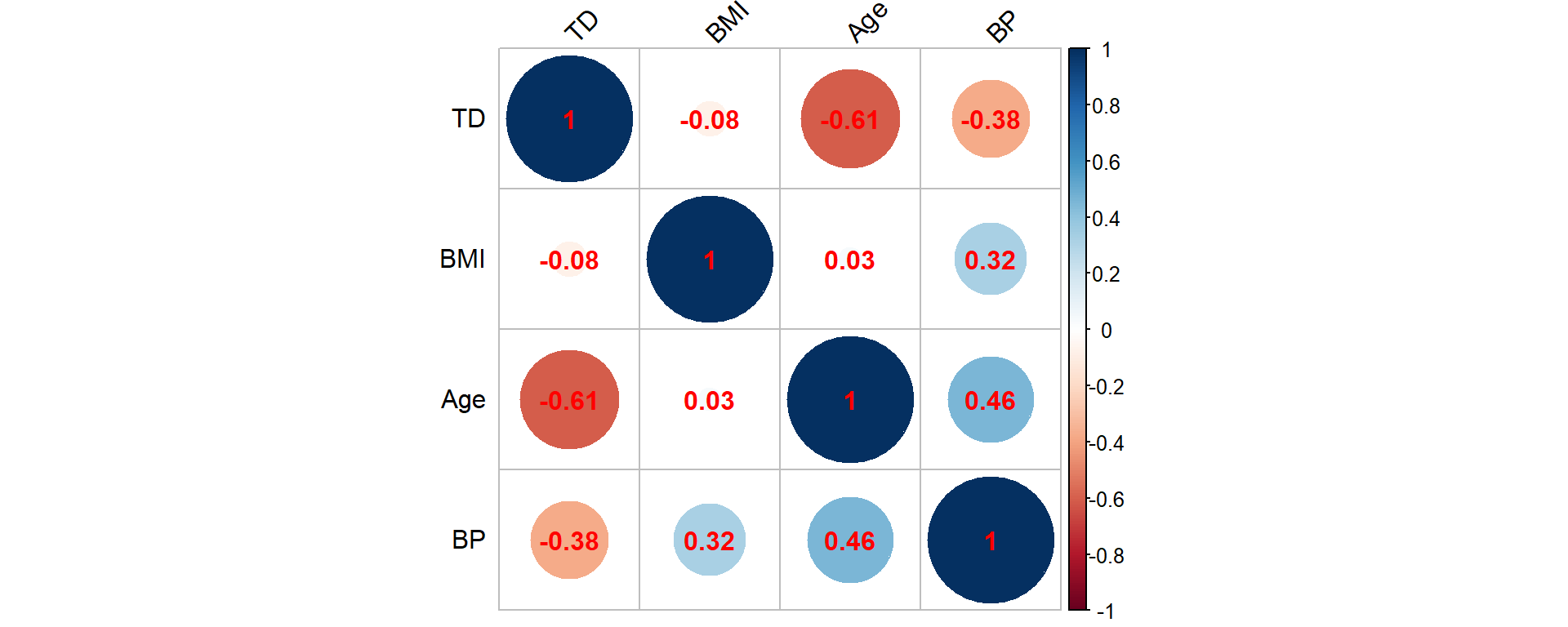
Figure 2.9: Correlation matrix for the synthetic mortality data corresponding to age, BMI, BP (blood pressure) and TD (time of death)

Hence, the time of death is (strongly) negatively associated with age, which is not surprising as elderly individuals are more likely to die. Similar patterns are also observed for the BMI and blood pressure attributes that are negatively associated with the time of death, but we should clarify that the BMI and blood pressure measurements are observed at policy inception. Nonetheless, these negative associations explain why such attributes are good predictors of the insured’s health. The pairwise correlation between age, BMI, and blood pressure are in line with our findings from Figure 2.6 that includes all insureds irrespective of their life status.

Even this simple analysis helps in understanding why the life office should evaluate the individual risk per policy by taking into consideration the available information.

Returning to our general description of survival data sets in the current context, if there was a claim and the death event was recorded, this data entry is non-censored; however, if the claim is not raised, then the policyholder is alive by the end of the observation period, and in turn, this datum is right-censored as the death event has not yet occurred. For example, consider a policyholder of age \(33\) that buys a policy in early January 1990, i.e. her/his Month_of_Sale record would be \(421\) – recall that month \(780\) indicates that a policy is bought in December 2019. If the policyholder survives to the end of the observation period, then a censored datum will be recorded as \(30\); in contrast, if the policyholder dies 13 years and 2 months after, then an uncensored datum will be recorded with an event time \(13+2/12\approx13.17\).

2.2 Modeling Death

The previous section introduced various examples of mortality data. Clearly, the most relevant question to actuaries is how to use the available pieces of information in order to devise lifetime models that could become the basis for analyzing the life-contingent exposures. This section provides the theoretical foundation for modeling lifetimes.

An important caveat is that we focus, both in the presentation of the datasets and in the modeling considerations in this chapter, on understanding the lifetime uncertainty for a given individual or (sub)population, where the life status is assumed to be dichotomous, i.e. alive and dead are the only life status under observation. This assumption helps us in creating a parsimonious presentation that is fit for its purpose at this very moment, though one could consider multi-state models – with multiple life status such as alive, death, temporary disability, permanent disability, and any other long term health condition, etc. – or models with multiple decrements that relate to specific life insurance products where the modeler could consider non-health related factors such as early termination of a contract that have an impact on the policy’s cashflows. Clearly multi-state and multi-decrement models present a generalization of the dichotomous lifetime model, where there are only two states – alive and dead – and a single decrement – dying, respectively. However, aside from being an important special case, there are benefits to discussing and building such more general models armed with the understanding of and experience working with the dichotomous model. We will return to multi-decrement and multi-state models in Chapter 6.

We commence by introducing the most important concept of a lifetime random variable and then discuss key actuarial quantities that allow for a formal interpretation of the data previously presented. We deviate from a traditional actuarial presentation in that we allow for general attributes, which we denote by \(\bf{x}\), to affect the lifetime distribution. However, towards the end of the section, we specialize to the more limited – but in traditional actuarial modeling conventional – assumption that the only relevant (dynamic) covariate for the distribution of the lifetimes is age \(x\).

2.2.1 Lifetime Random Variable and its Distribution

We start by considering an individual with attributes \(\bf{x}\) from some feature space. We assume that the attributes \(\bf{x}\) are sufficient to determine the distribution of the individual’s future lifetime, which we denote by \(T_{\bf{x}}\). In other words, the lifetime random variable \(T_{\bf{x}}\) follows a distribution depending on the attributes \(\bf{x}\). We will assume this random variable has positive real values, i.e. its support is \((0,\infty)\), and that the random variable is “well-behaved” (integrable, continuous, etc.) so that all the operations in what follows are well-defined.

It is helpful to pause and reflect on different types of possible attributes. Some attributes, such as the individual’s race, the individual’s (biological) sex, race, learned profession, etc., are immutable. Thus, one can either include them in the considered set of attributes \(\bf{x}\). Or we can consider a population of individuals with the same immutable characteristics, and then differentiate them solely by non-immutable characteristics \(\bf{x}\). The life expectancy tables in Section 2.1.1 serve as an example: here the relevant population could be hispanic females, for which we distinguished (only) different age levels. This approach, where age – typically denoted by \(x\) – is the only attribute under consideration, is the setting contemplated in traditional life-contingent analysis, and we will discuss this as an important special case in the last part 2.2.3 of this section.

However, this ``age-only" setting is restrictive from a number of perspectives. For instance, there are various individual characteristics that are relevant to the future lifetime that are non-immutable. For instance, the health-related attributes of BMI and systolic blood pressure in the dataset presented in Section 2.1.3 may change over time, and a blood pressure level of 130 for a 30 year old may carry a different interpretation than a level of 130 for a 70 year old. Moreover, environmental or socio-economic conditions may change over time and could impact the distribution of future lifetimes, and these could also be reflected in the set of attributes \(\bf{x}\). We leave the exploration of different relevant examples to the remaining sections of this chapter as well as later, more advanced chapters of this book.

Let \(F_{\bf{x}}\) and \(S_{\bf{x}}\) be the cumulative distribution function (cdf) and survival function of \(T_{\bf{x}}\), respectively: \[ F_{\bf{x}}(t) =\Pr(T_{\bf{x}}\le t)\quad \text{and}\quad S_{\bf{x}}(t) =\Pr(T_{\bf{x}} > t)=1-\Pr(T_{\bf{x}} \le t)=1-F_{\bf{x}}(t)\quad\text{for all}\;t\geq0. \]

Given our natural assumption that the lifetime variable \(T_{\bf{x}}\) is continuously distributed, i.e. that there are no outcomes that carry point masses, we can also defined its probability density function \(f_{\bf{x}}\):

\[ f_{\bf{x}}(t) =\frac{\partial F_{\bf{x}}(t)}{\partial t}=\frac{\partial \big(1- S_{\bf{x}}(t)\big)}{\partial t}=-\frac{\partial S_{\bf{x}}(t)}{\partial t},\;t\geq 0. \]

Similarly, we can define the force of mortality, \(\mu_\bf{x}\), which in different contexts is also referred to as the hazard rate or the mortality intensity:

\[ \mu_{\bf{x}}(t) = - \frac{\partial \log\{ S_{\bf{x}}(t)\}}{\partial t} = \frac{-\frac{\partial S_{\bf{x}}(t)}{\partial t}}{S_{\bf{x}}(t)}=\frac{f_{\bf{x}}(t)}{S_{\bf{x}}(t)},\;t\geq 0, \]

which is equivalent to: \[ S_{\bf{x}}(t) = \exp\left\{-\int_0^t \mu_{\bf{x}}(s)\;ds \right\}\quad\text{for all}\quad t\ge 0. \] The important point to note is that any one of the functions \(F_{\bf{x}}\), \(S_{\bf{x}}\), \(f_{\bf{x}}\), or \(\mu_{\bf{x}}\) completely determines the distribution of the future lifetime \(T_{\bf{x}}\). In other words, in order to specify a probabilistic model of future lifetimes, we can choose to model any of these quantities – knowing the form of just one of them will allow you to determine expressions for the other functions.

2.2.2 Standard Actuarial Notation: \(q_{\bf{x}}\), \(_tp_{\bf{x}}\), and All That

The introduction of the lifetime random variable, in principle, is enough for actuarial analyses of life-contingent exposures. In particular, as we will see in the next chapter, based on \(T_{\bf{x}}\) we can model (discounted) cash flows of common life insurance and annuity products, determine their expected values and variances, etc. However, the discussion so far was primarily formal and did not instill much intuition. For instance, the cdf \(F_{\bf{x}}(t)\) at time \(t\) is nothing else than the probability that an individual will die before a certain time \(t\), i.e. the mortality probability; and the expected value of \(T_{\bf{x}}\) is nothing else than the expected years lived, i.e. the life expectancy, for an individual with attributes \(\bf{x}\) that we had already encountered in Section 2.1.1 in the context of national vital statistics.

To instill interpretation into the notation, but also to have a precise, uniform representation to record and communicate relevant quantities, actuaries around the globe rely on so-called standard actuarial notation. This notation is based on a so-called Halo system where symbols are placed as superscript or subscript before or after a main character. In particular, the \(t\)-year mortality probability for an individual with attributes \(\bf{x}\) is denotes by \(_tq_{\bf{x}}\): \[ {_tq_{\bf{x}}} = F_{\bf{x}}(t),\;t\geq 0. \] Similarly the \(t\)-year survival probability, denoted by \(_tp_{\bf{x}}\), is nothing else than the survival function: \[ {_tp_{\bf{x}}} = S_{\bf{x}}(t),\;t\geq 0. \] Clearly, \({_tp_{\bf{x}}}+{_tq_{\bf{x}}}=1\), since the individual \(x\) either dies or survives after \(t\) units of time. Furthermore, is is conventional to drop a superscript of one: \[ {_1p_{\bf{x}}} = {p_{\bf{x}}}\quad\text{and}\quad {_1q_{\bf{x}}} = {q_{\bf{x}}}. \]

We denote the \(s\)-year mortality probability after surviving for \(t\) years as: \[ {_{t|s}q_{\bf{x}}} = F_{\bf{x}}(t+s) - F_{\bf{x}}(t) = {_{t+s}q_{\bf{x}}} - {_tq_{\bf{x}}} = S_{\bf{x}}(t) - S_{\bf{x}}(t+s) = {_tp_{\bf{x}}} - {_{t+s}p_{\bf{x}}} ,\;t,s\geq 0. \]

As indicated, the expected value of the lifetime random variable corresponds to the (complete) expectation of life or life expectancy. It is defined as follows:

\[ \stackrel{\circ}{e}_{\bf{x}}=E[T_{\bf{x}}]=\int_0^\infty t \,f_{\bf{x}}(t)\;dt=\int_0^\infty {_tp_{\bf{x}}}\;dt, \] where the last equaility follows from integration by parts.

Derivation of Formula for Complete Life Expectancy

\[ \stackrel{\circ}{e}_{\bf{x}} = E[T_{\bf{x}}] = \int_0^{\infty} t\, \underbrace{f_{\bf{x}}(t)}_{-S_{\bf{x}}'(t)}\,dt = - \left[S_{\bf{x}}(t)\, t\right]_{t=0}^{\infty} + \int_0^{\infty} S_{\bf{x}}(t)\,dt = \int_0^{\infty} {_tp_{\bf{x}}}\,dt. \]

It is also helpful to define a temporary version of the expectation of life, i.e. the number of years lived wihin the next \(n\) years. In actuarial notation, temporary quantities are denoted by \(\cdot_{\cdot:\overline{n}|}\): \[ \stackrel{\circ}{e}_{{\bf{x}}:\overline{n}|} = E[\min\{T_{\bf{x}},n\}] = \int_0^{n} {_tp_{\bf{x}}}\,dt. \] The interpretation is that unlike for the complete expectation of life, we only count years lived until time \(n.\) For instance, considering a population of \(l_0\) individuals, while \(l_0 \times {_tp_{\bf{x}}}\) denotes the expected number of survivors until time \(t\), \(l_0 \times \stackrel{\circ}{e}_{{\bf{x}}:\overline{t}|}\) denotes the average size of the population over the next \(t\) periods. We will return to this point in the context of life tables in section 2.4.

We will see many more examples of actuarial notation through the course of this book, and we will heavily rely on it.

2.2.3 The Classical Case: Age-Only Model

As mentioned, an important special case is the situation where the only (non-immutable) attribute is age. In this case, it is conventional to write \({\bf{x}} = x\), where \(x\) is a number denoting current age, and the lifetime random variable \(T_x\) that denotes the remaining future lifetime for an individual currently aged \(x\). Hence, in this case, \(T_x\) – and its distribution – solely depends on the age \(x\), and, thus, \(T_x\) and \((T_0-x)|T_0>x\) are identically distributed random variables (here \((T_0-x)|T_0>x\) denotes the random variable \(T_0 -x\) conditional on the event \(\{T_0>x\}\)). In other words, the future lifetime for \((x)\) is the same as the remaining future lifetime of a newborn given that this newborn reaches age \(x\), \(T_0>x\).

The mathematical formulations are thus described by conditional probabilities: \[\begin{eqnarray*} {_tq_x} = F_x(t) &=& Pr(T_x \le t) = Pr(T_x \le t \mid T_x>0) \\ &=& Pr(T_0-x \le t \mid T_0-x>0) = Pr(T_0 \le x + t \mid T_0 > x)\\ &=&\frac{\Pr(x<T_0\leq x+t)}{\Pr(T_0>x)}=\frac{F_0(x+t)-F_0(x)}{S_0(x)}=\frac{S_0(x)-S_0(x+t)}{S_0(x)} \end{eqnarray*}\] and \[\begin{eqnarray*} {_tp_x} = S_x(t) &=& Pr(T_x > t) = Pr(T_x > t \mid T_x > 0) \\ &=& Pr(T_0-x > t \mid T_0-x>0) = Pr(T_0 > x+t \mid T_0>x)\\ &=&\frac{\Pr(T_0> x+t)}{\Pr(T_0>x)}=\frac{S_0(x+t)}{S_0(x)}. \end{eqnarray*}\] Similarly, the probability density function of \(T_x\) is simply given by the conditional density function of \(T_0\): \[ f_x(t)=-\frac{\partial S_x(t)}{\partial t}=-\frac{\partial \left(\frac{S_0(x+t)}{S_0(x)}\right)}{\partial t}=-\frac{\frac{\partial S_0(x+t)}{\partial t}}{S_0(x)}=\frac{f_0(x+t)}{S_0(x)}\quad\text{for all}\;t>0, \] and the force of mortality: \[ \mu_x(t) = -\frac{\partial}{\partial t} \log\{S_x(t)\} = -\frac{\partial}{\partial t} \log\{S_0(x+t)\} = \mu_0(x+t) = \mu_{x+t}, \] i.e. it depends on current age only.

Given the formula for the survival probability, we have: \[ {_tp_x} = \frac{S_0(x+t)}{S_0(x)} = \frac{S_0(x+t)}{S_0(x+s)} \frac{S_0(x+s)}{S_0(x)} = \frac{S_0(x+s + (t-s))}{S_0(x+s)} \frac{S_0(x+s)}{S_0(x)} = {_{t-s}p_{x+s}}\,{_sp_x}, \] i.e. survival probabilities factorize into sub-period survival probabilities in this case. This is one of the key properties that does not hold in the general situation for \({_tp_{\bf{x}}}\) from the previous section, but simplifies expressions in this “age-only” model case. For instance, we obtain for the \(s\)-year mortality probability after surviving for \(t\) years as: \[ {_{t|s}q_{x}} = {_tp_x} - {_{t+s}p_x} = {_tp_x}\, (1 - {_sp_{x+t}}) = {_tp_x}\,{_sq_{x+t}},\;t,s\geq 0. \] As for another example, we can express the \(n\)-year temporary life expectancy for an \(x\)-year old as a function of complete life expectancies at ages \(x\) and \(x+n\), and the survival probability: \[ \stackrel{\circ}{e}_{x:\overline{n}|} = \stackrel{\circ}{e}_{x}-{_np_x}\,\stackrel{\circ}{e}_{x+n}. \]

Derivation of Relationship for Temporary Life Expectancy

\[ \stackrel{\circ}{e}_{x:\overline{n}|} = \int_0^{n} {_tp_x}\,dt = \int_0^{\infty} {_tp_x}\,dt - \int_n^{\infty} {_tp_x}\,dt = \stackrel{\circ}{e}_{x} - {_np_x}\,\int_n^{\infty} {_{t-n}p_{x+n}}\,dt = \stackrel{\circ}{e}_{x} - {_np_x}\,\int_0^{\infty} {_{t}p_{x+n}}\,dt = \stackrel{\circ}{e}_{x}-{_np_x}\,\stackrel{\circ}{e}_{x+n}. \]

Some of the most common models for future lifetimes fall in this category of “age-only models.” In particular, the most common analytical mortality laws that we will encounter in the next section as well as models based on conventional life tables (see Section 2.4) are ``age-only models" – both of which are very common in actuarial analysis. While the idea of age being the sole co-variate appears limiting, recall the note from above that one could view the model as specific to a certain population with the same immutable characteristics. Indeed, sometimes it is helpful to carry immutable characteristics as an additional subscript, say \({\bf{x}}=(x,a)\) where \(a\) is immutable. Here, the same considerations apply as in the “age-only model,” e.g. we have: \[ {_tp_{(x,a)}} = {_{t-s}p_{(x+s,a)}}\,{_sp_{(x,a)}}. \]

We will encounter similar models and notation in the context of select-and-ultimate life tables or in the context of cohort life tables in Section 2.4. That said, approaches that allow for individual attributes affecting the future lifetime distribution such as survival regression models that we will discuss in Section 2.6; or models that incorporate a stochastic evolution of mortality rates due to uncertainty in the demographic environment or in medical technology do not fall in this class of “age-only models,” but are covered by our more general approach and notation.

Obviously, in order to make the model accurate, it should include all possible sources of data and their attributes that could better differentiate the mortality risk amongst insureds. However, the choice of an appropriate model also depends on context and potential restrictions. For example, the use of genetic specific attributes for risk classification is under vast scrutiny by insurance ethical experts, since such pieces of information could lead to genetic discrimination, and therefore, there are regulatory constraints in using such attributes. Moreover, even the (biological) sex attribute – one of the most important mortality explanatory variable – is not always acceptable; for example, the European Union insurance regulations imposes pricing neutrality with respect to sex factors for quite some time, which means that life and non-life insurance policies issued within the European Union market should price males and females at the same level if all other observable attributes are similar.

We will return to such considerations in future chapters when contemplating instututional aspects of certain insurance products or services. In the remainder of this chapter, we will discuss the most common mortality models, i.e. ways of characterizing the distribution of \(T_{\bf{x}}\). In addition to its specification, we will also comment on statistical estimation of the resulting model.

2.3 Analytical Laws of Mortality

Early on, mortality modeling had focused on simplified parametric models that depend on few parameters and are known as Analytic Mortality Laws; such models assume simple analytic survival or mortality functions, which have their own merits though the lack of sophistication becomes visible quickly. Nonetheless, these models still illustrate key basic patterns, they provide tools for exploratory or “back-of-the envelope” actuarial calculations, and, from the pedagogical perspective, they present helpful “toy models” that aide in getting acquainted with actuarial modeling. These models typically fall in the category of “age-only” models from Section 2.2.3, so that a suitable interpretation is that the model describes the mortality of a specific population.

2.3.1 De Moivre and Constant Force Models

Starting with the simplest approach, it is clear that any survival function takes the value 1 and 0 at the left and right end point of its domain, respectively. Thus, if a newborn is assumed to have a known limiting age \(\omega\), then \(S_0(0)=1\) and \(S_0(\omega)=0\). One simple analytical example is the De Moivre Mortality Law which assumes a linear pattern for \(S_0\), i.e. \[ S_0(x) = 1 - \frac{x}{\omega}\quad\text{for all}\quad 0 \leq x \leq \omega. \] Now, the force of mortality becomes \[ \mu_x= \frac{-S_0'(x)}{S_0(x)} = \frac{\frac{1}{\omega}}{1 - \frac{x}{\omega}} = \frac{1}{\omega - x}\quad\text{for all}\quad 0 \leq x < \omega. \] This implies that if the lifetime distribution of a newborn follows De Moivre Mortality Law, then once the newborn reaches a certain age \(x\), the new lifetime distribution also follows De Moivre, with a parameterization replacing \(\omega\) with \(\omega -x\).

A generalization of the above analytical mortality law is known as the generalized De Moivre Law, and corresponds to a survival function with the following parametrization \[ S_0(x) = \left(1 - \frac{x}{\omega}\right)^{\alpha}\quad\text{for all}\quad 0\leq x \leq \omega, \] where the positive shape parameter \(\alpha\) decides how far the survival function departs from the linear dependence. Then, its force of mortality becomes \[ \mu_x = \frac{\alpha/\omega\,(1-x/\omega)^{\alpha-1}}{(1-x/\omega)^{\alpha}} = \frac{\alpha}{\omega - x}\quad\text{for all}\quad 0\leq x \leq \omega. \] Future lifetime distribution is also preserved with generalized De Moivre Law. For a newborn with mortality that follows this law, the future lifetime distribution, upon reaching a particular age \(x\), also follows generalized De Moivre Law. The \(\alpha\) parameter is preserved but as in De Moivre Mortality Law, parameter \(\omega\) is replaced with \(\omega -x\).

As indicated, a different approach is to impose a particular structure to the force of mortality. The simplest example is to consider a constant force of mortality model, i.e. \(\mu_t=\mu\) for all \(t>0\), which corresponds to an Exponentially distributed lifetime \(T_x\) with \[ S_0(x) = e^{-\mu\,x}\quad\text{for all}\quad x\ge 0. \] Note that this constant force mortality model does not square with the idea that mortality is increasing as a function of age, which makes it a poor candidate for modeling human mortality – although it may be a suitable candidate of modeling the death or failure of non-organisms. For the De Moivre and generalized De Moivre mortality laws, we do observe an increasing force of mortality, although the hyperbolic relationship also does not match typical patterns of human mortality.

2.3.2 Gompertz and Makeham Laws

In contrast, a candidate that is able to better depict human mortality is provided by the Gompertz Mortality Law and is given as follows: \[ \mu_x = B\cdot c^x \quad\text{for all}\quad x\ge 0\quad\text{with}\quad B>0,\,c>1. \] Its survival function becomes: \[ S_0(x) =\exp\left\{-\int_0^x \mu_t\;dt \right\}=\exp\left\{ - \frac{B}{\log(c)} (c^x - 1)\right\}\quad\text{for all}\quad x\ge 0. \]

Derivation of the Gompertz Survial Function

\[ \exp\left\{-\int_0^x \mu_t\;dt \right\}=\exp\left\{-\int_0^x B\cdot c^t\;dt \right\}=\exp\left\{-\frac{B \cdot c^t}{\log c}\Big\lvert_{t=0}^{t=x} \right\} =\exp\left\{ - \frac{B}{\log(c)} (c^x - 1)\right\}. \]

A three parameter version of the Gompertz Mortality Law was proposed by Makeham, where an age-independent term is added and captures the external causes of death, i.e.

\[ \mu_x = A + B\cdot c^x\quad\text{for all}\quad x\ge 0\quad\text{with}\quad B>0,\,A+B\geq 0,\,c>1, \] and is known as the Gompertz-Makeham Mortality Law or Makeham Mortality Law. Then, its survival function immediately follows as:

\[ S_0(x) = \exp\left\{-\int_0^x \mu_t\,dt\right\} = \exp\left\{ - Ax - \frac{B}{\log(c)} (c^x - 1)\right\}. \]

2.3.3 Makeham Law based on Life Expectancies Data

The Gompertz-Makeham mortality model is sufficiently rich to represent typical patterns in human mortality. To have workable models for applications for the remainder of the book, we fit the model to our life expectancy data from Section 2.1.1.

Formally, we interpret the given life expectancies as (generalized) moments of our model, and then rely on the (generalized) methods of moments (GMM) to pin down the model parameters. We omit statistical details behind GMM (see e.g. this introduction for more details), but intuitively we determine the model parameters that produce model moments that are closest, in the least-squares sense, to the given data. We can then appraise the model fit by analyzing how close the fitted model moments are to the actual moments.

In doing so, we define functions that determine the survival functions and the life expectancy at a given age \(x\), where we evaluate the associated integral numerically. We then run a numerical optimization procedure that determines the parameters that best approximate the empirical moments.

R Code For Estimating the Gompert model

S_0 <- function(x,A,B,c) { exp(- A * x - B * (exp(c*x) - 1)/ c) }

le <- function(age,A,B,c){
  Sfixed <- function(x){ S_0(x+age,A,B,c)/S_0(age,A,B,c)}
  res <- integrate(Sfixed,lower = 0, upper = (120-age))$value
  return(res)
}

tomin <- function(x){
  res <- 0
  for (i in 1:5){
    res <- res + (us_les[i,4] - le((i-1)*20,0.0001*(1+x[1]/100),0.000007*(1+x[2]/100),0.11*(1+x[3]/100)))^2
  }
  return(res)
}
library(pracma)
res <- fminsearch(tomin,c(0,0,0))
A_opt_fem <- A*(1+res$xmin[1]/100)
B_opt_fem <- B*(1+res$xmin[2]/100)
c_opt_fem <- c*(1+res$xmin[3]/100)

# Resulting parameters:
Sex <- c("Female","Male")
A <- c(0.0005385767,0.0008564071)
B <- c(1.119213e-05,3.544491e-05)
c <- c(0.1031558,0.09276854)
MakehamUS <- data.frame(Sex,A,B,c)

Here are the resulting parameters (note that, slightly abusing notation, we write \(c\) for \(\log\{c\}\) from the previous section):

kable(MakehamUS, digits = 7, format.args = list(big.mark = ","))

Sex	A	B	c
Female	0.0005386	0.0000112	0.1031558
Male	0.0008564	0.0000354	0.0927685

which match the U.S. life expectancies quite well. For instance, for the female life expectancies we obtain:

R Code For Deriving the Gompertz life expectancies

tmp <- us_les[,c(1,4)]
tmp$fitted <- rep(0,5)
for (i in 1:5){
  tmp[i,3] <- le((i-1)*20,MakehamUS$A[1],MakehamUS$B[1],MakehamUS$c[1])
}

kable(tmp, digits = 2, format.args = list(big.mark = ","))

Age	Female	fitted
0	81.1	81.05
20	61.8	61.87
40	42.6	42.72
60	24.7	24.49
80	9.8	9.90

and the following resulting survival function:

R Code For Figure

par(mfrow=c(1,2))
plot(MakehamUS$A[1] + MakehamUS$B[1] * exp(MakehamUS$c[1]*(1:120)), type = "l", lwd = 3, col = "blue", main = "Gompertz-Makeham Force of Mortality", xlab = "age", ylab = "mu")
plot(S_0(1:120,MakehamUS$A[1],MakehamUS$B[1],MakehamUS$c[1]), type = "l", lwd = 3, col = "green", main = "Gompertz-Makeham Survival Curve", xlab = "age", ylab = "S_0")

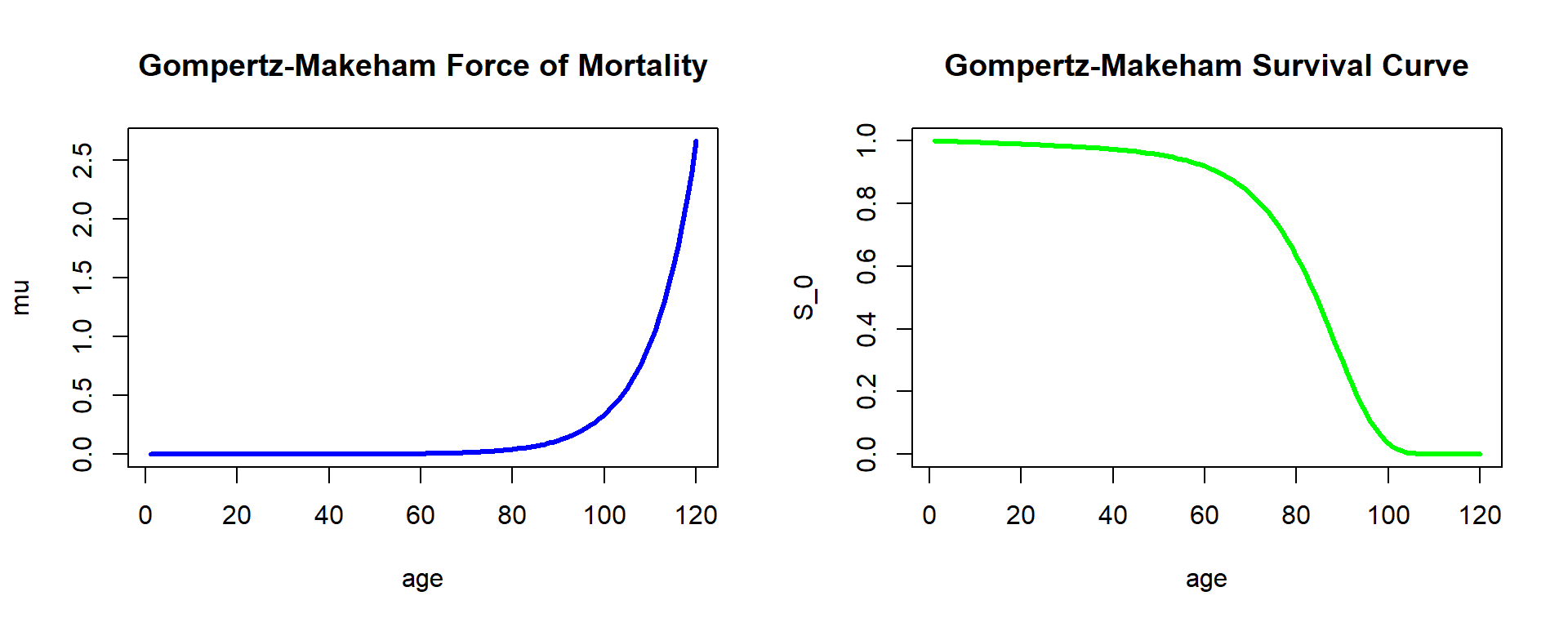
Figure 2.10: Fitted Force of Mortality and Survival Curve

2.4 Life Tables and their Functions

As we illustrated in the previous section, the Gompertz-Makeham model is able to describe basic mortality patterns quite well – and particularly match life expectancies across ages. However, the resulting force of mortality that is described by three parameters is highly regular. In particular, the likelihood of dying is monotonically increasing over the entire age domain. While this is true across many ages, real-world human mortality often shows a few deviations from these regular patterns. For instance, we often observe a so-called “young adult mortality hump” arising from risky behavior, involvement in wars, etc.

While there exist mortality laws that can account for this and other features, resulting functions quickly become complex and exhibit a low degree of tractability. Hence, a typical approach is to directly specify the survival function \(S_0(\cdot)\) of the lifetime random variable of a newborn within the “age-only” model and use it for actuarial calculations. Such an approach is often characterized as non-parametric since the survival function is not given as a function of a few given parameters. We will discuss more advanced approaches to estimating non-parametric survival functions from mortality data in Section 2.5.

A rather simple approach in this direction is to construct so-called life tables. As we discuss in the first part of this chapter, a life-table is simply an annually-discretized version of the survival function \(S_0(\cdot)\). A substantial advantage is that it is easy to generate such life tables in the context of population count data that we encountered in Section 2.1.2, as we will see and do in the second section 2.4.2. The following sections 2.4.3 and 2.4.4 then discuss in more detail the theoretical underpinnings of life tables based on the so-called curtate lifetime and how to derive quantities for fractional ages based on the annually-discretized representation. Finally, the concluding section 2.4.5 discusses more advanced, two-dimensional life tables that include mortality improvements. We will encounter similar structures in later chapters when discussing how to account for underwriting (selection) effects within so-called select-and-ultimate tables.

2.4.1 Life Table Basics

Consider a (large) population of \(l_0\) homogeneous newborns. Then, if survival in the population follows (exactly) the survival function \(S_0(\cdot)\), at age \(x\) there are: \[ l_0 \times S_0(x) = l_0 \times {_xp_0} = l_0 \times P(T_0 \geq x) = l_x \] individuals left. Of course, this immediately implies \({_xp_0} = \frac{l_x}{l_0}\) and, similarly, we can derive the \(k\)-year survival probability for an \(x\)-year old as: \[ {_kp_x} = \frac{S_0(x+k)}{S_0(x)} = \frac{l_0 \times S_0(x+k)}{l_0 \times S_0(x)} = \frac{l_{x+k}}{l_x},\,x,k=0,1,2,... \] In particular, the set of \(l_x,\,x=0,1,2,...,\) lets us compute relevant probabilities for integer choices, which is not surprising because they are effectively providing an annually-discretized version of the survival function \(S_0(\cdot)\) in the age-only model. Evidently the so-called radix \(l_0\) is immaterial, although it is typically chosen as a large number in line with the population interpretation, so that it is not necessary to display too many decimal digits. A life table provides exactly the set of \(l_x,\,x=0,1,2,...,\) typically compiled in a tabular manner starting at some initial age (maybe zero for a population table) up to some terminal age \(\omega\) after which all individuals are assumed to have died, i.e., \(l_{\omega + 1} = 0.\)

From the above equation, we immediately obtain: \[ {_kq_x} = 1 - {_kp_x} = \frac{l_x - l_{x+k}}{l_x} = \frac{_kd_x}{l_x},\,x,k=0,1,2,... \] where \(_kd_x\) denotes the deaths between ages \(x\) and \(x+k\). In particular, we have: \[ q_x = 1 - p_x = \frac{d_x}{l_x} \Leftrightarrow l_x - l_x\times p_x = d_x \Leftrightarrow l_{x+1} = l_x\times p_x = l_x - d_x,\,x=0,1,2,... \]

This suggests one way of creating a life table: We could observe a (large) cohort of \(l_0\) individuals initially, count the annual deaths \(d_0,\) \(d_1,\) etc., and tabulate the resulting survivors. The result would be a so-called cohort life table as it reflects survivorship of the observed cohort over time. However, this approach is rather unpractical: we would have to wait until the last person in the cohort has deceased, and by then compiling a life table for an extinct cohort is likely of limited use.

The more common approach is to compile a so-called period life table. Here instead of following a particular cohort, we consider a given population over a certain period, e.g. a calendar year. We then use observed population mortality rates \(q_x\) in the time period to determine \(l_x\) for all ages according to the relationship above. We explore this idea using the population mortality data we introduced in Section 2.1.2.

2.4.2 Life Table based on U.S. Population Data

In section 2.1.2 we considered exposures and deaths of the U.S. population over time, and in particular in Figure 2.3 we plotted mortality rates—defined as the fraction of deaths and exposures—referencing the similarity to the Gompertz-Makeham law from Figure 2.10. It may be tempting to think about this mortality rates as \(q_x\) and use it to compile a life table. However, while the two quantities are related, there is a subtle difference: the mortality probability \(q_x = d_x/l_x\) considers deaths during age \(x\) relative to the population of \(x\) year olds.

In contrast, the central death rate is defined as the number of deaths each year that have characteristics \(\bf{x}\) at the moment of death in the relevant observation period, divided by the exposures with the same characteristics \(\bf{x}\) over the same period, and is denoted as \(m_\bf{x}\)—where as usual we write \(m_{x}\) in the age-only model. Hence, in particular the denominator corresponds to the average size of the population at risk, not the population at risk at the outset.

To connect \(q_x\) and \(m_x\), we need to make an assumption about the exposure. One straightforward approach is to assume that the exposures correspond to the arithmetic average of the population size at age \(x\) and the population size at age \(x+1\), though different approaches are possible as we will see in Section 2.4.4: \[ m_x \approx \frac{d_x}{0.5\,l_x+ 0.5\,l_{x+1}} = \frac{q_x}{1-0.5\,q_x} \Longrightarrow q_x = \frac{2\,m_x}{2+m_x}. \]

Let us use this relationship to construct a mortality life table using the 2010-2014 U.S.Females and Males data:

us_mx <- us_deaths 
us_mx[,4:6] <- us_deaths[,4:6] / us_exp[,4:6]
us_mx_fem_2014 <- us_mx[us_mx$Year_start == 2010,-c(2,5,6)]
colnames(us_mx_fem_2014)[colnames(us_mx_fem_2014)=="Female"] <- "mx US Females"
us_mx_fem_2014$qx <- 2 * us_mx_fem_2014$mx / (2 + us_mx_fem_2014$mx)
colnames(us_mx_fem_2014)[colnames(us_mx_fem_2014)=="qx"] <- "qx US Females"
tmp_head_us_mx_fem_2014 <- head(us_mx_fem_2014); rownames(tmp_head_us_mx_fem_2014) <- NULL
kable(head(tmp_head_us_mx_fem_2014), align = "ccr")

Year_start	Age	mx US Females	qx US Females
2010	0	0.005461737	0.005446862
2010	1	0.000379927	0.000379855
2010	2	0.000224890	0.000224865
2010	3	0.000169394	0.000169380
2010	4	0.000138322	0.000138313
2010	5	0.000119244	0.000119237

us_mx_mal_2014 <- us_mx[us_mx$Year_start == 2010,-c(2,4,6)]
colnames(us_mx_mal_2014)[colnames(us_mx_mal_2014)=="Male"] <- "mx US Males"
us_mx_mal_2014$qx <- 2 * us_mx_mal_2014$mx / (2 + us_mx_mal_2014$mx)
colnames(us_mx_mal_2014)[colnames(us_mx_mal_2014)=="qx"] <- "qx US Males"
tmp_head_us_mx_mal_2014 <- head(us_mx_mal_2014); rownames(tmp_head_us_mx_mal_2014) <- NULL
kable(head(tmp_head_us_mx_mal_2014), align = "ccr")

Year_start	Age	mx US Males	qx US Males
2010	0	0.006554279	0.006532870
2010	1	0.000441664	0.000441567
2010	2	0.000298869	0.000298824
2010	3	0.000225097	0.000225072
2010	4	0.000184733	0.000184715
2010	5	0.000145992	0.000145981

The death probability curves for the U.S. Females and Males data are depicted in both original and logarithmic scales, and displayed as Figure ??.

R Code For Figure

par(mfrow=c(2,2))
plot(us_mx_fem_2014$qx,type = "l", lwd = 5, col = "blue", main="Original scale Female", xlab = "age", ylab = "q_x",ylim = c(0,1.0))
lines(us_mx_fem_2014$mx,col="red")
plot(log(us_mx_fem_2014$qx, base = 10),type = "l", lwd = 5, col = "blue", main="Log scale Female", xlab = "age", ylab = "q_x")
plot(us_mx_mal_2014$qx,type = "l", lwd = 5, col = "blue", main="Original scale Male", xlab = "age", ylab = "q_x",ylim = c(0,1.0))
lines(us_mx_mal_2014$mx,col="red")
plot(log(us_mx_mal_2014$qx, base = 10),type = "l", lwd = 5, col = "blue", main="Log scale Male", xlab = "age", ylab = "q_x")

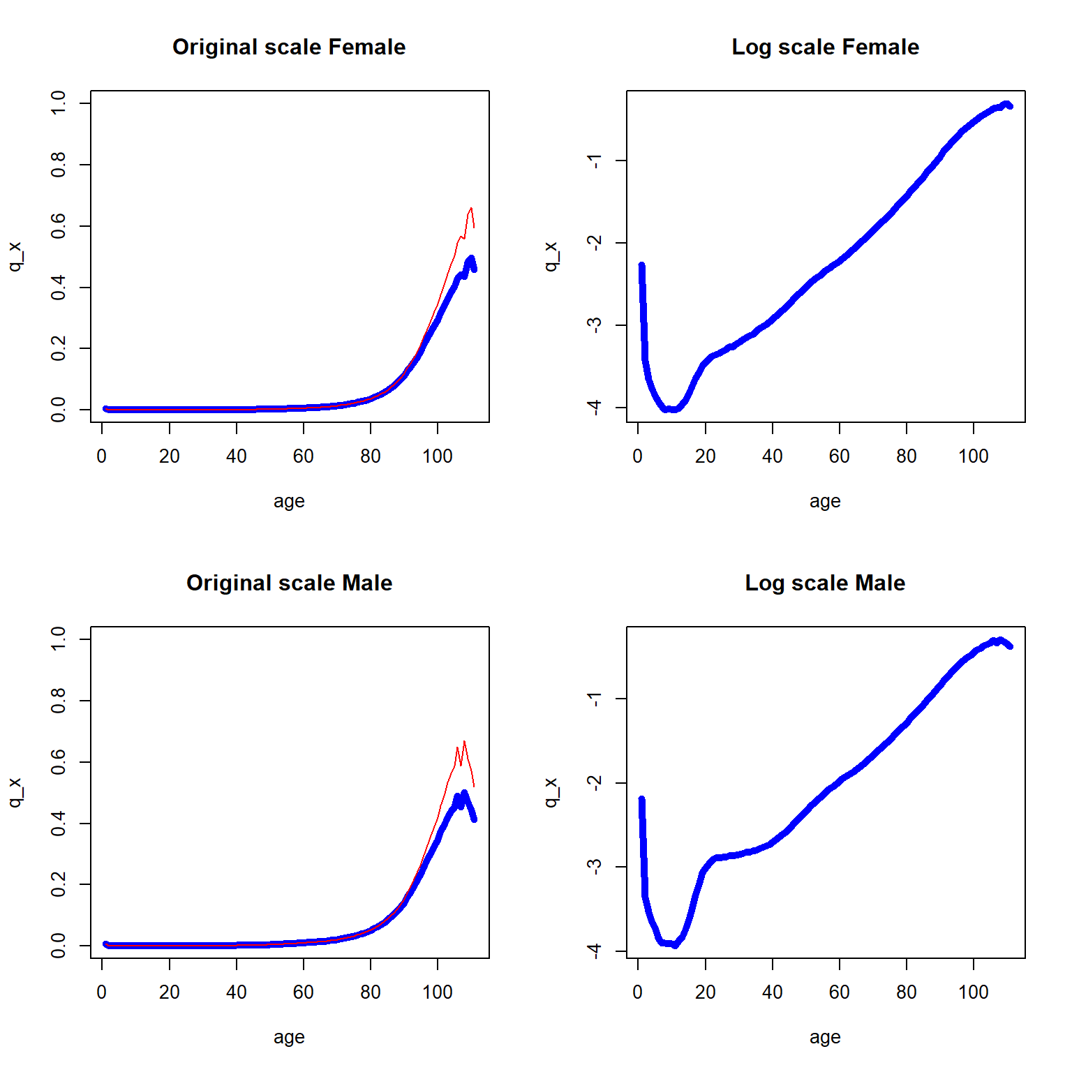
Figure 2.11: One year death probability curve (in blue) and central death rate (in red) for the 2010-2014 U.S. data across all ages

As we can see, \(q_x\) and \(m_x\) are similar with the exception of the later years. As expected, the log scale plots are more informative in the sense that the log scale reveals the marginal changes over various ages, and we now combined the two log scaled curves into Figure 2.12.

R Code For Figure

par(mfrow=c(1,1))
plot(log(us_mx_fem_2014$qx, base = 10), type = "l", lwd = 5, col = "blue", main="Log scale", xlab = "age", ylab = "q_x")
lines(log(us_mx_mal_2014$qx, base = 10), lwd = 5, col = "red")

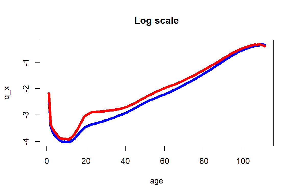
Figure 2.12: One year death probability curve for the 2010-2014 U.S. Females (in blue) and Males (in red) data across all ages

Figure 2.12 shows the usual higher mortality rates for males than for females, but also extremely pronounced differences at ages 16 to 40 that could be explained by social factors that are specific to U.S. Males at post adolescence ages. As indicated before, these intricacies are not accounted for by the Gompertz-Makeham and other simple parametric models. Moreover, significant differences at ages 50 to 70 are also observed, and are due to health related factors that males around the world tend to be exposed earlier than females.

We are now able to construct a period life table based on the U.S. mortality data. Using the relationships from before: \[ l_{x+1}=l_x\cdot p_x=l_x\big(1-q_x\big)\quad\text{for all integers}\quad x. \] and fixing \(l_0 = 1,000,000\), we generate \(l_x\), \(x=0,1,2,...\), for the male and female life table:

lf <- rep(0,length(us_mx_fem_2014$mx))
lf[1] <- 1000000
for (i in 2:111){
  lf[i] = lf[i-1] * (1-us_mx_fem_2014[i-1,4]) 
}
us_mx_fem_2014$lf <- lf

lm <- rep(0,length(us_mx_mal_2014$mx))
lm[1] <- 1000000
for (i in 2:111){
  lm[i] = lm[i-1] * (1-us_mx_mal_2014[i-1,4])
}
us_mx_mal_2014$lm <- lm

Resulting in, for females:

library(DT)
tmp_life_table_us_mx_fem_2014 <- round(us_mx_fem_2014, digits = 9); 
colnames(tmp_life_table_us_mx_fem_2014)[5]<- "lx US Females"

rownames(tmp_life_table_us_mx_fem_2014) <- NULL
#kable(tmp_life_table_us_mx_fem_2014, digits = 9, format.args = list(big.mark = ","), align = "ccrrr")
DT::datatable(tmp_life_table_us_mx_fem_2014)

And for males:

tmp_life_table_us_mx_mal_2014 <-round(us_mx_mal_2014, digits = 9); 
colnames(tmp_life_table_us_mx_mal_2014)[5]<- "lx US Males"
rownames(tmp_life_table_us_mx_mal_2014) <- NULL
#kable(tmp_life_table_us_mx_mal_2014, digits = 9, format.args = list(big.mark = ","), align = "ccrrr") 
DT::datatable(tmp_life_table_us_mx_mal_2014) 

The \(l_x\) values are now plotted in Figure 2.13 where once again the female subpopulation shows higher survivorship trend than the male subpopulation.

R Code For Figure

plot(lf, type = "l", lwd = 5, col = "yellow", xlab = "age", ylab = "l_x",ylim = c(0,1000000))
lines(lm, type = "l", lwd = 5, col = "orange", xlab = "age", ylab = "l_x",ylim = c(0,1000000))

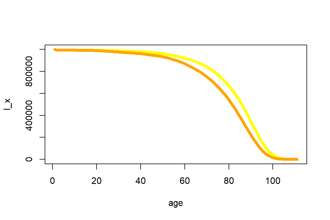
Figure 2.13: Expected number at risk for the 2010-2014 U.S. Females (in yellow) and Males (in orange) data across all ages

There are more advanced approaches to fine-tune the life table, e.g. by smoothing approaches to adjust small deviations in the observed mortality data. However, when relying on the sizable U.S. population, the resulting quantities are fairly smooth as illustrated by Figures 2.12 and 2.13. Hence, we will rely on them without adjustments.

We can rely on the life table to determine various actuarial quantities, at integer ages and for integer durations. For instance, we can determine the survival probabilities \(_kp_{50}\) for a 50-year-old female for all choices of \(k=0,1,2,...\):

kP50 <- us_mx_fem_2014$l[51:111]/us_mx_fem_2014$l[51]

R Code For Figure

plot(kP50,xlab="age", type = "l", lwd = 5, col = "red")

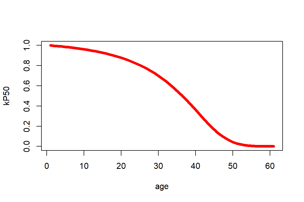
Figure 2.14: kPx for a 50-year old female

Or we can determine \(_{10|20}q_{50}\), the probability that a 50-year old survives for 10 years and then dies within the next 20 years via \(\frac{l_{60}-l_{80}}{l_{50}}\):

(us_mx_fem_2014$l[61] - us_mx_fem_2014$l[81])/us_mx_fem_2014$l[51]

[1] 0.281351377

2.4.3 Curtate Quantities and Recursive Relationships

Rather than thinking about life tables as an annually-discretized version of the survival function of \(T_0\) within the age-only model, it is also possible to interpret a life table as providing probabilities of a discretized version of the lifetime random variable. This is referred to as the curtate future lifetime.

Formally, the curtate future lifetime \(K_{\bf{x}}\) is given by the greatest integer of \(T_{\bf{x}}\): \(K_{\bf{x}} = \lfloor T_{\bf{x}} \rfloor\), i.e.
\[\begin{eqnarray*} K_{\bf{x}} = 0 & \text{ if } & T_{\bf{x}} < 1\\ K_{\bf{x}} = 1 & \text{ if } & 1\leq T_{\bf{x}} < 2\\ &...&\\ K_x = {\bf{x}} & \text{ if } & k \leq T_{\bf{x}} < k+1,\, k \in {\mathbb N}. \end{eqnarray*}\] Therefore, \(K_{\bf{x}}\) describes the number of whole future years lived by an individual with characteristics \({\bf{x}}\) prior to death. Therefore, the probability function of the (discrete) distribution of \(K_{\bf{x}}\) is: \[ Pr(K_{\bf{x}} = k) = Pr(k \leq T_{\bf{x}} < k+1) = {_kp_{\bf{x}}} - {_{k+1}p_{\bf{x}}} = {_{k\mid 1}q_{\bf{x}}} = {_{k\mid}q_{\bf{x}}},\,k=0,1,... \]

Just as for the lifetime, the expected value of \(K_x\) corresponds to a life expectancy, though this is a curtate version of life expectancy. It is denoted by \(e_{\bf{x}}\), and its calculation can be obtained by summing up the \({_kp_{\bf{x}}}\) in analogy to the derivation of (complete) life expectancy: \[ e_{\bf{x}} = E[K_{\bf{x}}]= \sum_{k=1}^{\infty} {_kp_{\bf{x}}}. \]

Derivation of Formula for Curtate Life Expectancy

\[\begin{eqnarray*} e_{\bf{x}} &=& E[K_{\bf{x}}] = \sum_{k=0}^{\infty} k \, Pr(K_{\bf{x}}=k) = \sum_{k=0}^{\infty} k\, ({_kp_{\bf{x}}} - {_{k+1}p_{\bf{x}}}) \\ &=& \sum_{k=0}^{\infty} k\, {_kp_{\bf{x}}}-\sum_{k=0}^{\infty} (k+1)\, {_{k+1}p_{\bf{x}}} + \sum_{k=0}^{\infty} {_{k+1}p_{\bf{x}}}\\ &=&\sum_{k=1}^{\infty} {_kp_{\bf{x}}}. \end{eqnarray*}\]

As before, in the age-only model we write \({\bf{x}}=x\), and in this case we can express the curtate expected lifetime of an \(x\)-year old by the corresponding value for an \(x+1\) year old: \[\begin{eqnarray*} e_x &=& \sum_{k=1}^{\infty} {_kp_x} = p_x \,\sum_{k=1}^{\infty} {_{k-1}p_{x+1}} = p_x\,{_0p_{x+1}} + p_x\,\sum_{k=2}^{\infty} {_{k-1}p_{x+1}} \\ &=& p_x + p_x \sum_{i=1}^{\infty} {_{i}p_{x+1}} = p_x + p_x \cdot e_{x+1} \end{eqnarray*}\] or \[ e_{x} = p_x\left(1+e_{x+1}\right) \Leftrightarrow e_{x+1} = \frac{e_x - p_x}{p_x}. \] This recursive formula states that the expected future lifetime for an \(x\)-year-old in whole years will be non-zero for the survivors until age \(x+1\) only, and for those it will be the expected future lifetime in whole years for an \(x+1\)-year-old individual plus the one year they already have survived.

Curtate life expectancies are straightforward to calculate from a life table. For instance, using our life table for females, we obtain for curtate life expectancy at birth is:

kP0f <- us_mx_fem_2014$l/us_mx_fem_2014$l[1]
e_0 <- sum(kP0f) - 1
e_0

[1] 80.7955575

which is close to the Figure from the U.S. national statistics from Section 2.1.1, where the female life expectancy for 2017 is recorded as 81.1 years. We are also now in a position to elaborate on the caveat at the end of that section on the interpretation of this number: This is a so-called period life expectancy as it was derived from a period life table. So rather than reflecting the prospective life expectancy of a newborn today, it describes how long a hypothetical newborn that will have the mortality patterns observed in the population within this period will be expected to live. We will attempt to derive a more representative figure for a 50-year old alive today that will experience future mortality rates in Section 2.4.5.

Indeed, an interesting and revealing exercise is to go through past years of data that we have available in our population count data from Section 2.1.2, and derive life expectancies for past periods. We consider newborn and fifty-year-old females. We obtain this by essentially repeating the same exercise we carried out in the previous section to assemble the life table for every time period.

R Code For Figure

e0 <- rep(0,16)
e50 <- rep(0,16)

i <- 1

for (s in seq(1935,2010,5)){
  #Get central death rates for each start year
  mx <- us_mx[us_mx$Year_start == s,4]
  S0 <- rep(0,111)
  
  #Calculate the survival function
  S0[1] <- 1
  for (j in 2:111){
    S0[j] <- S0[j-1]*(1 - (2*mx[j-1])/(2 + mx[j-1]))
  }

  #And evaluate curtate life expectancies by summing over kPx's
  e0[i] <- sum(S0) - 1
  e50[i] <- sum(S0[51:111]/S0[51]) - 1
  i <- i+1
}

par(mfrow=c(1,2))
plot(seq(1935,2010,5),e0, type = "l", lwd = 5, col = "blue", main="life expectancies at birth, across years", xlab = "year", ylab = "life expectancy")
plot(seq(1935,2010,5),e50, type = "l", lwd = 5, col = "red", main="life expectancies at 50, across years", xlab = "year", ylab = "life expectancy")

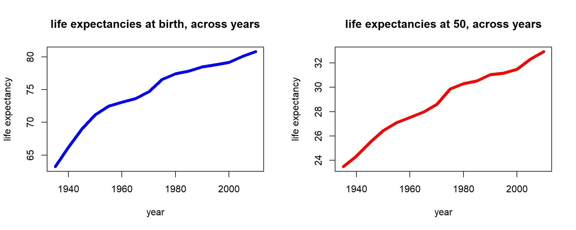
Figure 2.15: Female life expectancies across time for U.S. females

We notice that period life expectancies have consistently increased, and indeed the increase seems close to linear. This is a familiar observation from demography, where it is pointed out that various limits on life expectancy that were previously assumed have been broken.

2.4.4 Fractional Year Assumptions

Let us consider the complete life expectancy in the age-only model for an \(x\)-year old life or, more precisely, the recursive relationship: \[\begin{eqnarray*} \stackrel{\circ}{e}_{x} &=& \int_0^{\infty} {_tp_x}\,dt = \int_0^{1} {_tp_x}\,dt +\int_1^{\infty} {_tp_x}\,dt = \int_0^{1} {_tp_x}\,dt +p_x\,\int_1^{\infty} {_{t-1}p_{x+1}}\,dt \\ &=& \underbrace{\int_0^{1} {_tp_x}\,dt}_{e_{\overline{x:1|}}} +p_x\,\stackrel{\circ}{e}_{x+1}. \end{eqnarray*}\] In order to derive the life expectancy from a life table with a terminal age \(\omega\), we could rely on this recursion. Clearly \(\stackrel{\circ}{e}_{\omega}=0\), so to derive \(\stackrel{\circ}{e}_{x}\) for \(x=\omega-1,\,\omega-2,...,1,0\), we can employ the \(p_x\) as denoted in the life table. However, we also need to compute \(\int_0^{1} {_tp_x}\,dt\) and, thus, we need to know how \(_tp_x\) evolves within one year or, in other words, for . The common way in actuarial practice to solve this problem, but also to derive quantities like \({_{1.5}p_{55}}\) or \({_{10}q_{22.5}}\), is to use interpolation schemes, i.e. to make an assumption on the distribution of \(S_0(x)\)—or, equivalently, \(l_x\)—between integers.

One of the most common assumptions is that of a uniform distribution of deaths within each year of age (UDD). To illustrate, note that the number of deaths within the population of \(x\)-year olds is \[ d_x = l_x \times q_x. \] The UDD assumption is that in, say, half of the year, half of the people die; similarly, say, in a third of the year, a third of the people die, i.e.
\[\begin{eqnarray*} {_{0.5}d_x} &=& 0.5\times d_x, \\ {_{0.333}d_x} &=& 0.333 \times d_x \end{eqnarray*}\] or, in general, \[ {_{t}d_x} = t\times d_x, \;0\ \leq t \leq 1, \] which implies \[ {_tq_x} = \frac{_td_x}{l_x} = t \frac{d_x}{l_x} = t\times q_x, \;0\ \leq t \leq 1. \] Of course, we can also express this relationship in terms of the survival function: \[\begin{eqnarray*} \frac{S_0(x) - S_0(x+t)}{S_(x)} = {_tq_x} &=& t\cdot q_x = t\;\frac{S_0(x) - S_0(x+1)}{S_0(x)} \\ \Rightarrow S_0(x+t) &=& S_0(x) + t \left(S_0(x+1) - S_0(x)\right), \;0\ \leq t \leq 1. \end{eqnarray*}\] Thus, this assumption is equivalent to assuming a linear interpolation of the survival function bewteen integers.

Based on the survival function and the familiar relationships, we can now derive all other actuarial quantities in terms of the discrete amount of quantities denoted in the life table; for example, for the survival probability we obtain: \[ {_tp_x} = 1- {_tq_x} = 1 - t\times q_x, \;0\ \leq t \leq 1; \] and for the force of mortality: \[\begin{eqnarray*} \mu_{x+t} &=& \frac{-S_0'(x+t)}{S_0(x+t)} = \frac{-\frac{\partial}{\partial t}{_{x+t}p_0}}{{_{x+t}p_0}} \\ &=& \frac{{_xp_0}\,\left(-\frac{\partial}{\partial t}{_tp_x}\right)}{{_xp_0}\,{_{t}p_x}} = \frac{q_x}{1-t\cdot q_x}, \;0\ \leq t \leq 1. \end{eqnarray*}\]

In order to determine probabilities for fractional starting ages, let us first consider the probability to die within the second part of some given year, i.e. \(_{1-t}q_{x+t}\), \(0\ \leq t \leq 1:\) the probability to die before age \(x+1\) for some \(x+t\) year old life, where \(x\) is integer valued. The probability to survive for \(t\) periods and to then die within the remaining \(1-t\) periods plus the probability to die within the first \(t\) periods clearly must equal the probability to die within the whole year, i.e.
\[ {_tp_x} \times {_{1-t}q_{x+t}} + {_tq_x} =\frac{S_0(x+t)}{S_0(x)}\frac{S_0(x+t) - S_0(x+1))}{S_0(x+t)} + \frac{S_0(x)-S_0(x+t)}{S_0(x)} = \frac{S_0(x) - S_0(x+1)}{S_0(x)} = {q_x} \] and, therefore: \[ {_{1-t}q_{x+t}} = \frac{q_x - t\times q_x}{_tp_x} = \frac{(1-t)\times q_x}{1-t\times q_x}. \] For the probability to die before age \(x+t+u\) for an \((x+t)\)-year old life, where \(0 \leq u < 1-t\), we can rely on the same reasoning as above: In the \((1-t)\) time periods between age \(x+t\) and \(x+1\), a proportion of \(_{1-t}q_{x+t}\) of the entire population die. Thus, in the first \(u\) time periods, \(\frac{u}{1-t}\) as many people will die, i.e. \[ {_{u}q_{x+t}} = \frac{u}{1-t} {_{1-t}q_{x+t}} = \frac{u}{1-t}\frac{(1-t)\,q_x}{1-t\,q_x} = \frac{u\,q_x}{1-t\,q_x}. \] However, we could have also simply relied on the interpolation scheme for \(S_0(x)\) and applied the familiar formulas.

Finally, for the integral within the recursion for the life expectation, we have \[ \int_0^1 {_tp_x}\,dt = \int_0^1 1 - t\,q_x\,dt = 1 - q_x \left.\frac{1}{2}t^2\right|_{t=0}^1 = \frac{1 + p_x}{2}. \] Note that this implies that under the UDD assumption: \[ m_x = \frac{d_x}{\int_0^1 l_{x+s}\,ds}=\frac{l_x\,q_x}{l_x\,\int_0^1 {_tp_x}\,dt} = \frac{q_x}{1-0.5\,q_x}, \] which is exactly the relationship we used in relating \(m_x\) and \(q_x\) in the previous section to construct our life table. That is, we implictly relied on a UDD assumption. Similarly, connecting to our motivational example, under UDD we obtain: \[ \stackrel{\circ}{e}_{x} = \frac{1}{2} + e_x, \] so that our observations for the curtate life expectancies will closely resemble those for the complete life expectancies.

Derivation of Relationship between Curtate and Complete Life Expectancy under UDD

\[\begin{eqnarray*} \stackrel{\circ}{e}_{x} &=& \frac{1}{2} + \frac{1}{2}\,p_x + p_x \,\stackrel{\circ}{e}_{x+1} = \frac{1}{2} + p_x\,(\frac{1}{2}+\stackrel{\circ}{e}_{x+1})\\ &=& \frac{1}{2} + p_x\,(\frac{1}{2}+\frac{1}{2} + \frac{1}{2}\,p_{x+1} + p_{x+1} \,\stackrel{\circ}{e}_{x+2}) = \frac{1}{2} + p_x + {_2p_x}\,(\frac{1}{2}+\stackrel{\circ}{e}_{x+2})\\ &=& ...\\ &=& \frac{1}{2} + \sum_{k=1}^{\inft} {_kp_x} = \frac{1}{2} + e_x. \end{eqnarray*}\]

An alternate common assumption is that the force of mortality remains constant over the year (constant force assumption): \[ p_x = e^{-\int_0^1 \mu_{x+t}\,dt} = e^{-\mu_x}, \] where \(\mu_{x+t} = \mu_{x},\;0 \leq t < 1\), which immediately yields \[ \mu_{x+t} = \mu_x = -\log\left\{p_x\right\},\;0 \leq t < 1, \] and, hence: \[ {_tp_x} = e^{-\int_0^t \mu_{x+t}\,dt} = e^{-\mu_x\,t} = p_x^t. \] This, on the other hand, implies: \[\begin{eqnarray*} \frac{S_0(x+t)}{S_0(x)} &=& \left(\frac{S_0(x+1)}{S_0(x)}\right)^t \\ \Rightarrow \; S_0(x+t) &=& S_0(x)\left(\frac{S_0(x+1)}{S_0(x)}\right)^t,\;0\leq t < 1, \end{eqnarray*}\] so we are looking at an scheme.

Clearly, all other quantities can now again be derived on the basis of \(S_0(x+t)\). In particular, for the central death rate, we obtain: \[ m_{x}=\frac{q_x}{\int_0^1 {_tp_x}\;dt}=\frac{1-e^{-\mu_x}}{\int_0^1 e^{-\mu_x \,t}\;dt}=\frac{1-e^{-\mu_x}}{\big(1-e^{-\mu_x}\big)/\mu_x}=\mu_x, \] yielding the relationship: \[ q_x = 1-e^{-\mu_{x}} = 1-e^{-m_x}. \] This is an alternate, similarly common way of connecting \(q_x\) and \(m_x\) in constructing life tables. The differences are relatively minor.

2.4.5 Cohort Life Tables and Mortality Improvement Modeling

When compiling a period life table as we did in this chapter, we are relying on a snapshot of mortality experience for a given year or a given period. However, for a life insurance company selling annuities, in order to adequately price and reserve for their future liabilities, it is necessary to take into account future changes in mortality. As we have seen in Figure 2.15, life expectancies have changed substantially over the last decades. This means that a female born today may not have the same life expectancy \(e_{0}\) that we determined from our period life table (81.8, which as close to the U.S. national figure of 81.1 years)

One simple way of describing how mortality changed across years and ages are so-called mortality improvement factors, i.e. the percentage reduction in the mortality rate for each age \(x\) over successive years (\(t-1\) to \(t\)): \[ \varphi(x,t) = 1 - \frac{q_{x,t}}{q_{x,t-1}}. \] where now \(q_{x,t}\) is the mortality probability for an \(x\)-year-old at time \(t\). In particular, this is a deviation from the age-only model since we have a bivariate \({\bf{x}}=(x,t)\).

Let us consider mortality improvement factors in our dataset. Since we consider data in five-year intervals, we scale to one year: \[ \varphi(x,t) = 1 - \left(\frac{q_{x,t}}{q_{x,t-5}}\right)^{1/5}. \] One way of visualizing is a so-called heat map:

R Code For Figure

us_mx_fem <- us_mx[,-c(2,5,6)]
colnames(us_mx_fem)[colnames(us_mx_fem)=="Female"] <- "mx"
us_mx_fem$qx <- 1-exp(-us_mx_fem$mx)

phi <- matrix(rep(0,111*15),nrow=111,ncol=15,byrow = TRUE)
for (t in 1:15){
  for (x in 1:111){
    phi[x,t] <- 1 - (us_mx_fem[t*111+x,4]/us_mx_fem[(t-1)*111+x,4])^(1/5)
  }
}
heatmap(phi,Colv = NA,Rowv = NA,labCol = seq(1935,2010,5), xlab="Year", ylab="Age", main="Mortality Improvements")
legend(x="right", legend=c("low", "med", "high"),fill=heat.colors(3))

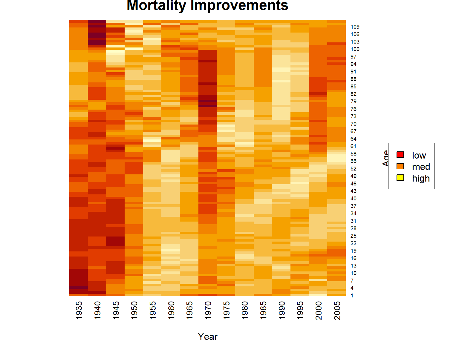
Figure 2.16: Heatmap for Mortality Improvements for U.S. Females Across Times and Ages

As we can see, mortality improvements vary quiet a bit over time and age, but we do see quite substantial improvements for low to medium ages in the more recent past. One interesting aspect here is that clearly there is a relationship between time and age. For a certain birth cohort, as time passes, the individuals will age. In particular, we identify the diagonals in the heatmap with a certain birth cohort, and we observe some distinct relationships on the diagonals. For instance, the cohort if individuals born around 1950 appears to experience quite substantial improvements across all years of age, which could be due to environmental or socio-economic factors.

One simple way of accounting for improvements and forecasting mortality into the future are so-called single factor mortality improvement models, i.e. models where \(\varphi(x,t)\) only depends on \(x\) – let’s write \(\varphi_x\). With that, the above equation becomes: \[ q_{x,t}= q_{x,t-1}\times (1- \varphi_x), \] or, generalizing: \[ q_{x,t} = q_{x,0}\times (1-\varphi_x)^t \]

To obtain suitable improvement factors for making projections, for deriving \(\phi_x\) let’s average across years under consideration and smooth across ages using a simple local regression smoother:

R Code For Figure

phi_x <- rep(0,111)
for (x in 1:111){
  phi_x[x] <- mean(phi[x,])
}
ages <- 1:111
lo <- loess(phi_x ~ ages)
plot(phi_x, type = "l", lwd = 5, col = "red", main="Mortality Improvement Factors, US Females", xlab = "age", ylab = "phi")
lines(predict(lo), col='blue', lwd=2)
phi_x <- predict(lo)

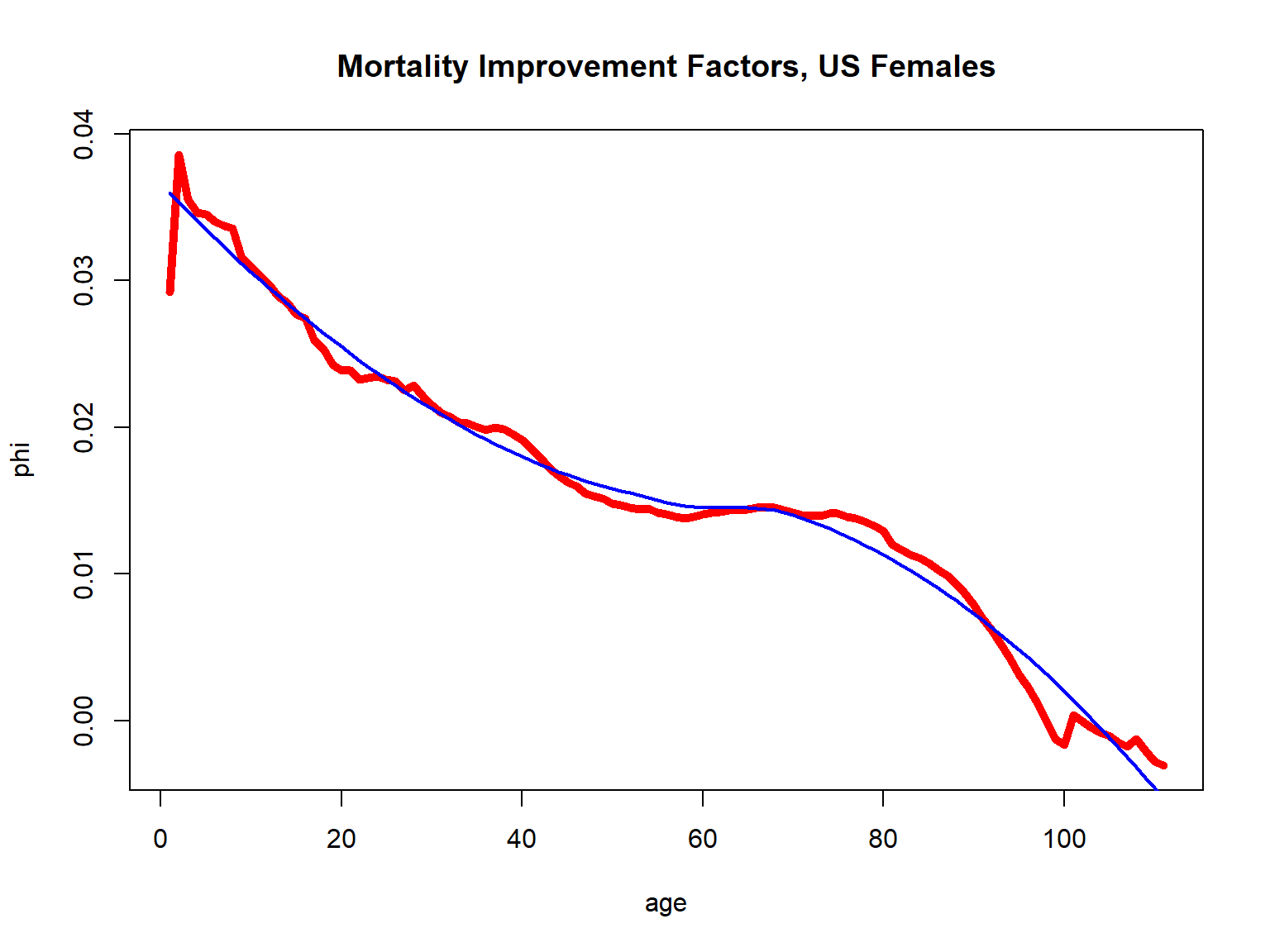
Figure 2.17: Mortality Improvement Factors for U.S. Females

It is important to stress that we are no longer in the age-only model, since now a seventy-year-old today and a seventy-year-old ten years from now. However, as we already indicated in Section 2.2.3, in this case of a bivariate \(\bf{x}\) where one of the covariates—year of birth—is immutable for an individual, we can still rely on the same ideas as in the age-only model. Hence, in particular, we can still defined life tables, although life tables will now be two dimensional since we will have different \(q_{x,t}\) for every year \(t\).

To illustrate, let us create a cohort life table for fifty year old females now, where for simplicity we denote the current time by \(t=0\) (corresponding to the timing of the period life table we created). Then we can obtain prospective mortality probabilities \(q_{50+t,t}\) via: \[ q_{50+t,t} = q_{50+t,0} \times (1-\varphi_{50+t})^t. \] Let us plot these cohort mortality probabilities and compare them to our period mortality probabilities:

R Code For Figure

q_50plusx <- rep(0,61)
for (i in 1:61){
  q_50plusx[i] <- us_mx_fem_2014[50+i,4] * (1 - phi_x[50+i])^(i-1)
}
plot(50:99,q_50plusx[1:50], type = "l", lwd = 2, col = "red", main="q_x comparison", xlab = "age")
lines(50:99,us_mx_fem_2014[51:100,4], col = "blue", lwd = 2)

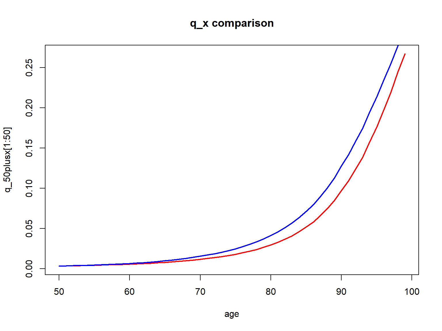
Figure 2.18: Cohort (red) vs. Period (blue) q_x for 50-year old U.S. females

Evidently the cohort mortality probabilities are lower than the period mortality probabilities, as we incorporate mortality improvements. Of course, this comes with the assumption that the future mortality evolution will be similar to that in the past. While critical, it is not possible to make a projections without any assumption, and reliance on a period table is equivalent to assuming there will not be improvements whatsoever. These \(q_{50+t,t}\) and now be relied on for determining actuarial quantities just as in the previous section.

If we use all ages \(x\) today and determine corresponding \(q_{x+t,t}\), \(t=0,1,2,...\), \(x=0,1,2,...\), just as above, we obtain a two-dimensional cohort or projective life table. In particular, we can consider newborn females and determine their (curtate) life expectancy, resulting in:

R Code For Cohort Life Expectancy

q_0plusx <- rep(0,110)
for (i in 1:110){
q_0plusx[i] <- us_mx_fem_2014[i,4] * (1 - phi_x[i])^(i-1)
}
kP0_i <- rep(0,110)
kP0_i[1] <- 1 
for (i in 2:110){
  kP0_i[i] <- kP0_i[i-1] * (1 - q_0plusx[i-1])
}
e_0Coh <- sum(kP0_i) - 1 

e_0Coh

[1] 88.1249429

Hence, due to mortality improvements, our projected life expectancy is substantially larger than that based on our period table of 80.8 years from Section 2.4.3 or that based U.S. national statistics of 81.1 from Section 2.1.1.

select-and-ultimate tables.

2.5 Non-parametric Survival Estimation

The previous section introduced life tables as a (discretized) representation of a non-parametric survival function in the age-only model. We also showed how to compile a period life table based on (population) mortality count data, essentially by deriving mortality rates from a given time window.

How can we determine a life table—or, more generally, a survival function—from mortality data at the individual level, which an insurance company has available, such as the dataset we introduced in Section 2.1.3? One approach is to follow a similar path as in the previous section, by translating the individual outcomes into counts and the proceeding similarly. However, the number of deaths within a given year and at a certain age may be rather limited for a single company’s portfolio, especially when constraining the individuals to a certain subgroup determined by sex, smoking status, health, etc. Therefore, in practice life tables are often compiled at the industry level, such as within the so-called Valuation Basic Table by the American Academy of Actuaries.

The current section discusses non-parametric estimation of survival functions based on a individual level mortality dataset that inlcudes truncated and censored data, where we rely on the dataset from Section 2.1.3 for illustration. In anaology to the previous section, the setting here is the age-only approach, i.e., we determine one survival curve that reflects mortality as a function of age. However, by constraining the dataset to certain subrgoups, we can generate different survival curves for these different subgroups. We commence by introducing the Kaplan-Meier (product limit) approach for estimating the survival curve and then discuss the Nelson-Aalen estimator for the cumulative hazard.

2.5.1 Kaplan-Meier Estimates

The intuition for the Kaplan-Meier estimate is straightforward. Recall from Section 2.2.3 that in the age-only model, for the survival function for \(x\)-year-olds we have: \[ S_x(0) = 1 \text{ and } S_x(t+1) = S_x(t) \times p_{x+t} \] for integer \(x\) and \(t\). Furthermore, from the previous section on life tables, given information on exposures \(l_{x+t}\) and deaths \(d_{x+t}\) at time \(x+t\), we estimate: \[ p_{x+t} = 1 - \frac{d_{x+t}}{l_{x+t}} \Longrightarrow S_x(t+1) = S_x(t) \times \left(1 - \frac{d_{x+t}}{l_{x+t}}\right). \] The Kaplan-Meier estimate uses the exact same relationship, although it takes into account that in the context of right-censored individual mortality data, potential exposures at each death time may be different. That is, \(l_{x+t}\) in this equation should be interpreted as the total number of individuals at risk of dying at time \(x+t\). This number will change across time because individuals die and because of right-censoring, so indviduals falling outside of the observation window. As a consequence, the survival function is updated whenever there is a death event, and the number of corresponding exposures is recalculated at every point. For additional details as well as a discussion of how to determine the variance of the estimate, we refer to Section 4.3.2 in Loss Data Analystics.

An important caveat to the application of the Kaplan-Meier estimate is that all exposures are treated alike in the context of the age-only model. Hence, individuals of the same age at different times are entering the survival curve estimate. In particular, the set of observations that is used for estimating the survival curve determines the population for which the survival curve is relevant.

In R, we can use the library survival. We estimate survival curves based on our insurer dataset from Section 2.1.3 for ages 30, 40, and 50, where we compare survival curves for males, females, and the aggregate curves. Let us plot them curves.

R Code For Figure

library(data.table)
library(survival)
insdatatmp <- fread("Data/SyntheticInsurerData.csv",data.table=FALSE)

# computations for individuals aged 50 
ageX <- 50
#FEMALE
sexX <- 0 # 0 for female, 1 for male
setdata <- insdatatmp[which(insdatatmp$Age+floor(insdatatmp$Time_of_death) >=ageX & insdatatmp$Age <= ageX & insdatatmp$Sex==sexX),]
time <- rep(0,nrow(setdata))
status<-1*(setdata$Claim == "YES") # 0 for Censored data observations (i.e. with no claims and Claim=="No"), 1 for non-Censored observations -- setting for Survfit function
time <- setdata$Time_of_death - (rep(ageX,nrow(setdata))-setdata$Age)
fit_KM_50_F <- survfit(Surv(time,status) ~ 1, type='kaplan-meier') # Kaplan-Meier estimator
#MALE
sexX <- 1 # 0 for female, 1 for male
setdata <- insdatatmp[which(insdatatmp$Age+floor(insdatatmp$Time_of_death) >=ageX & insdatatmp$Age <= ageX & insdatatmp$Sex==sexX),]
time <- rep(0,nrow(setdata))
status<-1*(setdata$Claim == "YES") # 0 for Censored data observations (i.e. with no claims and Claim=="No"), 1 for non-Censored observations -- setting for Survfit function
time <- setdata$Time_of_death - (rep(ageX,nrow(setdata))-setdata$Age)
fit_KM_50_M <- survfit(Surv(time,status) ~ 1, type='kaplan-meier')
#AGGREGATE
setdata <- insdatatmp[which(insdatatmp$Age+floor(insdatatmp$Time_of_death) >=ageX & insdatatmp$Age <= ageX),]
time <- rep(0,nrow(setdata))
status<-1*(setdata$Claim == "YES") # 0 for Censored data observations (i.e. with no claims and Claim=="No"), 1 for non-Censored observations -- setting for Survfit function
time <- setdata$Time_of_death - (rep(ageX,nrow(setdata))-setdata$Age)
fit_KM_50_All <- survfit(Surv(time,status) ~ 1, type='kaplan-meier')

# computations for individuals aged 40 
ageX <- 40
#FEMALE
sexX <- 0 # 0 for female, 1 for male
setdata <- insdatatmp[which(insdatatmp$Age+floor(insdatatmp$Time_of_death) >=ageX & insdatatmp$Age <= ageX & insdatatmp$Sex==sexX),]
time <- rep(0,nrow(setdata))
status<-1*(setdata$Claim == "YES") # 0 for Censored data observations (i.e. with no claims and Claim=="No"), 1 for non-Censored observations -- setting for Survfit function
time <- setdata$Time_of_death - (rep(ageX,nrow(setdata))-setdata$Age)
fit_KM_40_F <- survfit(Surv(time,status) ~ 1, type='kaplan-meier') # Kaplan-Meier estimator
#MALE
sexX <- 1 # 0 for female, 1 for male
setdata <- insdatatmp[which(insdatatmp$Age+floor(insdatatmp$Time_of_death) >=ageX & insdatatmp$Age <= ageX & insdatatmp$Sex==sexX),]
time <- rep(0,nrow(setdata))
status<-1*(setdata$Claim == "YES") # 0 for Censored data observations (i.e. with no claims and Claim=="No"), 1 for non-Censored observations -- setting for Survfit function
time <- setdata$Time_of_death - (rep(ageX,nrow(setdata))-setdata$Age)
fit_KM_40_M <- survfit(Surv(time,status) ~ 1, type='kaplan-meier')
#AGGREGATE
setdata <- insdatatmp[which(insdatatmp$Age+floor(insdatatmp$Time_of_death) >=ageX & insdatatmp$Age <= ageX),]
time <- rep(0,nrow(setdata))
status<-1*(setdata$Claim == "YES") # 0 for Censored data observations (i.e. with no claims and Claim=="No"), 1 for non-Censored observations -- setting for Survfit function
time <- setdata$Time_of_death - (rep(ageX,nrow(setdata))-setdata$Age)
fit_KM_40_All <- survfit(Surv(time,status) ~ 1, type='kaplan-meier')

# computations for individuals aged 30 
ageX <- 30
#FEMALE
sexX <- 0 # 0 for female, 1 for male
setdata <- insdatatmp[which(insdatatmp$Age+floor(insdatatmp$Time_of_death) >=ageX & insdatatmp$Age <= ageX & insdatatmp$Sex==sexX),]
time <- rep(0,nrow(setdata))
status<-1*(setdata$Claim == "YES") # 0 for Censored data observations (i.e. with no claims and Claim=="No"), 1 for non-Censored observations -- setting for Survfit function
time <- setdata$Time_of_death - (rep(ageX,nrow(setdata))-setdata$Age)
fit_KM_30_F <- survfit(Surv(time,status) ~ 1, type='kaplan-meier') # Kaplan-Meier estimator
#MALE
sexX <- 1 # 0 for female, 1 for male
setdata <- insdatatmp[which(insdatatmp$Age+floor(insdatatmp$Time_of_death) >=ageX & insdatatmp$Age <= ageX & insdatatmp$Sex==sexX),]
time <- rep(0,nrow(setdata))
status<-1*(setdata$Claim == "YES") # 0 for Censored data observations (i.e. with no claims and Claim=="No"), 1 for non-Censored observations -- setting for Survfit function
time <- setdata$Time_of_death - (rep(ageX,nrow(setdata))-setdata$Age)
fit_KM_30_M <- survfit(Surv(time,status) ~ 1, type='kaplan-meier')
#AGGREGATE
setdata <- insdatatmp[which(insdatatmp$Age+floor(insdatatmp$Time_of_death) >=ageX & insdatatmp$Age <= ageX),]
time <- rep(0,nrow(setdata))
status<-1*(setdata$Claim == "YES") # 0 for Censored data observations (i.e. with no claims and Claim=="No"), 1 for non-Censored observations -- setting for Survfit function
time <- setdata$Time_of_death - (rep(ageX,nrow(setdata))-setdata$Age)
fit_KM_30_All <- survfit(Surv(time,status) ~ 1, type='kaplan-meier')

# survival function plots
par(mfrow=c(1,3))
plot(fit_KM_30_F$surv~fit_KM_30_F$time,type="l", main="Kaplan–Meier Estimates at age 30", xlab="Time", ylab="Survival Function",col = "blue")
lines(fit_KM_30_M$surv~fit_KM_30_M$time,col = "red")
lines(fit_KM_30_All$surv~fit_KM_30_All$time,col = "green")
plot(fit_KM_40_F$surv~fit_KM_40_F$time,type="l", main="Kaplan–Meier Estimates at age 40", xlab="Time", ylab="Survival Function",col = "blue")
lines(fit_KM_40_M$surv~fit_KM_40_M$time,col = "red")
lines(fit_KM_40_All$surv~fit_KM_40_All$time,col = "green")
plot(fit_KM_50_F$surv~fit_KM_50_F$time,type="l", main="Kaplan–Meier Estimates at age 50", xlab="Time", ylab="Survival Function",col = "blue")
lines(fit_KM_50_M$surv~fit_KM_50_M$time,col = "red")
lines(fit_KM_50_All$surv~fit_KM_50_All$time,col = "green")

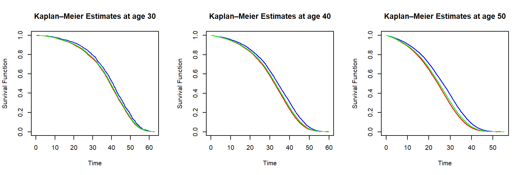
Figure 2.19: Kaplan-Meier survival function estimates for an individual of age 30 (left), 40 (middle) and 50 (right) based on the insurer dataset – curves are in blue (female), red (male) and green (all genders)

In line with results from the aggregate mortality data, Figure ?? tells us that females are more likely to survive over the same period than males. The curves for all genders are closer to the equivalent curves based on the male data, since the synthetic dataset has \(70\%\) male policyholders, as explained in the data summary given in Section 2.1.3.

2.5.2 Nelson-Aalen Estimates

The Nelson-Aalen estimator provides a non-parametric estimat of the cumulative hazard rate function \[ A_x(t) =\int_0^t \mu_x(s)\,ds. \] We have for the cumulative hazard rate: \[ S_x(t+1) = \exp\{-A_x(t+1)\}=S_x(t)\,\exp\{-(A_x(t+1)-A_x(t))\}=S_x(t)\,\frac{l_{x+t+1}}{l_{x+t}}. \]

To provide intuition for the Nelson-Aalen estimator, recall that for `small’ arguments, the exponential function \(e^y \approx 1 + y\). Therefore, we have: \[ 1 - (A_x(t+1)-A_x(t)) \approx \frac{l_{x+t+1}}{l_{x+t}} \Longrightarrow A_x(t+1) \approx A_x(t) + \frac{d_{x+t}}{l_{x+t}}. \] However, in analogy to the derivation of the Kaplan-Meier estimat, the Nelson-Aalen estimator takes into account that in the context of right-censored individual mortality data, potential exposures at each death time may be different. That is, \(l_{x+t}\) in this equation should be interpreted as the total number of individuals at risk of dying at time \(x+t\). This number will change across time because individuals die and because of right-censoring, so indviduals falling outside of the observation window. And, again, the estimator updates whenever there is a death event. The esimator thus amounts to nothing else than the sum of deaths over exposures. Again we refer to Section 4.3.2 in Loss Data Analystics for more information.

Using the library survival, we can also obtain Nelson-Aalen estimates of the survival curve. We estimate survival curves based on our insurer dataset from Section 2.1.3 for females and ages 30, 40, and 50.

R Code For Figure

sexX <- 0 # 0 for female, 1 for male
# computations for individuals aged 50 
ageX <- 50
setdata <- insdatatmp[which(insdatatmp$Age+floor(insdatatmp$Time_of_death) >=ageX & insdatatmp$Age <= ageX & insdatatmp$Sex==sexX),]
time <- rep(0,nrow(setdata))
status<-1*(setdata$Claim == "YES") # 0 for Censored data observations (i.e. with no claims and Claim=="No"), 1 for non-Censored observations -- setting for Survfit function
time <- setdata$Time_of_death - (rep(ageX,nrow(setdata))-setdata$Age)
fit_NA_50_F <- survfit(Surv(time,status) ~ 1, type='fleming-harrington') # Nelson–Aalen estimator

# computations for individuals aged 40
ageX <- 40
setdata <- insdatatmp[which(insdatatmp$Age+floor(insdatatmp$Time_of_death) >=ageX & insdatatmp$Age <= ageX & insdatatmp$Sex==sexX),]
time <- rep(0,nrow(setdata))
status<-1*(setdata$Claim == "YES") # 0 for Censored data observations (i.e. with no claims and Claim=="No"), 1 for non-Censored observations -- setting for Survfit function
time <- setdata$Time_of_death - (rep(ageX,nrow(setdata))-setdata$Age)
fit_NA_40_F <- survfit(Surv(time,status) ~ 1, type='fleming-harrington') # Nelson–Aalen estimator

# computations for individuals aged 30
ageX <- 30
setdata <- insdatatmp[which(insdatatmp$Age+floor(insdatatmp$Time_of_death) >=ageX & insdatatmp$Age <= ageX & insdatatmp$Sex==sexX),]
time <- rep(0,nrow(setdata))
status<-1*(setdata$Claim == "YES") # 0 for Censored data observations (i.e. with no claims and Claim=="No"), 1 for non-Censored observations -- setting for Survfit function
time <- setdata$Time_of_death - (rep(ageX,nrow(setdata))-setdata$Age)
fit_NA_30_F <- survfit(Surv(time,status) ~ 1, type='fleming-harrington') # Nelson–Aalen estimator

# survival function plots
par(mfrow=c(1,3))
plot(fit_NA_30_F$surv~fit_NA_30_F$time,type="l", main="Nelson-Aalen Estimates at age 30", xlab="Time", ylab="Survival Function",col = "blue")
plot(fit_NA_40_F$surv~fit_NA_40_F$time,type="l", main="Nelson-Aalen Estimates at age 40", xlab="Time", ylab="Survival Function",col = "blue")
plot(fit_NA_50_F$surv~fit_NA_50_F$time,type="l", main="Nelson-Aalen Estimates at age 50", xlab="Time", ylab="Survival Function",col = "blue")

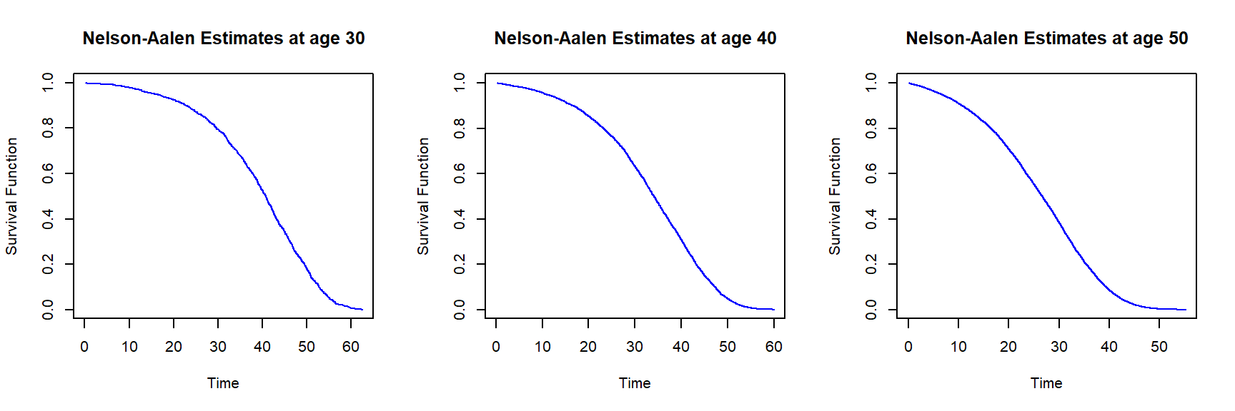
Figure 2.20: Nelson-Aalen survival function estimates for females of age 30 (left), 40 (middle) and 50 (right) based on the insurer dataset

Given that the dataset has a large sample size, the differences between the Kaplan-Meier and Nelson-Aalen estimates are insignificant; this is not surprising, since the two estimators are asymptotically equivalent – for large samples, the estimators are supposed to provide the same results.

Since the Kaplan-Meier and Nelson-Aalen estimators provide a full non-parametric estimate of the survival curve, we can directly use it for evaluating quantities depending on the distribution of the lifetime random variable. In principle, there is no need to discretize it to compile a life table – although that’s certainly possible. To reiterate, the approach in the application is to assemble a suitable set of lives and determine a survival function viewing these lives as a (sufficiently) homogeneous population. In the next section, we consider survival analysis models that explicitly account for the heterogeneity of individuals’ exposures by accounting for their characteristics.

2.6 Conditional Models: Survival regression

All models introduced in the foregoing sections 2.3 (analytic mortality laws), 2.4 (life tables based on mortality count data), and 2.5 (non-parametric estimates of the survival curve based on a homogeneous population) are based on the age-only model that – with some qualifications (see, e.g., Section 2.4.5). However, as introduced in Section 2.1.3, individual survival or event data that an insurance company has available consists of features or covariates \({\bf{x}}_i\) for each individual \(i\), plus the death time \(T_i\) if the individual had died or – if that’s not the case – the information that the individual is still alive. Hence, a proximate approach is to directly model the individual lifetime distribution \(T_{{\bf{x}}_i}\), i.e., to explicitly account for the heterogeneity in the individuals’ exposures. This can be accomplished via so-called survival regression models that predict the distribution of \(T_{{\bf{x}}}\) based on a set of features \({\bf{x}}_i\) and death times \(T_i\), \(i=1,2,\cdots,N\).

Our objective is to introduce some key ideas and to derive workable models. Therefore, we primarily focus on the most popular model – namely the proportional hazard (Cox) model – and consider linear models in the features. A detailed introduction of this rich set of models is beyond the scope of this text, although we note that in principle more sophisticated models can be used. We refer to the Notes and Comments section at the end of this chapter for references that go beyond our introduction.

We start by introducing the Cox proportional hazard model in the first part. We apply it to our individual level mortality dataset from Section 2.1.3 in the second part. And, finally, we show how to produce different models and life tables on the basis of the regression model.

2.6.1 The Cox Proportional Hazard Model

The task at hand is to formulate a model for the individual survival function \(S_{\bf{x}}(\cdot)\) given a feature vector \(\bf{x}\). Concretely, this may mean specifying a parametric model, i.e., to posit that \(S_{\bf{x}}(t)\) takes a certain functional form of time \(t\), the features \(\bf{x}\), and certain parameters, say \(\beta\). We can then try to estimate the parameters based on our data \(({\bf{x}}_i,T_i)_{1\leq i \leq N}\). However, a key challenge are the boundedness and monotonicity constraints for the survival function \(S_{\bf{x}}(\cdot)\).

Therefore, it is common in survival analysis to model the individual force of mortality (or hazard function) \(\mu_{\bf{x}}(\cdot)\). In principle, \(\mu_{\bf{x}}(t)\) can take any positive number, although as we had discussed in Section @ref{S:AnalMortLaws} a human’s force of mortality typically increases in age. Hence, a common approach in survival analysis is to posit that \(\mu_{\bf{x}}(t)\) takes a certain functional form of time \(t\), the features \(\bf{x}\), and parameters \(\beta\), and then try to estimate the parameters based on our data \(({\bf{x}}_i,T_i)_{1\leq i \leq N}\).

Different functional forms are possible. For example, additive survvial regression models specify \(\mu_{\bf{x}}(t)\) as a linear combination of the features, similarly to linear regression models. However, the most popular approach – due to its tractability and fit in many situations – is the so-called Cox proportional hazard model. In its simplest form, it assumes the force of mortality takes the form: \[ \mu_{\bf{x}}(t)=\beta_0(t) \times \exp\left\{ \beta' \,{\bf{x}}\right\}, \] in which \(\beta\) is the vector of regression parameters. The non-parametric term \(\beta_0(t)\) is also referred to as the parameter when the emphasis is on the estimation of the regression coefficients. It is also possible to allow for time-varying covariates: \[ \mu_{\bf{x}}(t) = \beta_0(t)\times\exp\left\{\beta'\, {\bf{x}}(t)\right\}, \] where \({\bf{x}}(t)\) are (possibly) time-varying covariates. Since the covariates are given, we in order to obtain (an estimate for) \(\mu_{\bf{x}}(t)\), we need to estimate the parameter vector \(\beta\). We outline the estimation process below, although the details are not crucial for the material that follows.

Estimation of the Regression Parameters in the Proportional Hazards Model

For a set of \(N\) independent subjects, define the observation time \(X_i = \min\{T_i, C_i\}\), \(i\in\{1,\ldots,n\}\), where \(T_i\) is time until death and \(C_i\) is the censoring time (time until end of observation period) for subject \(i\). The indicator for observed death of subject \(i\) is defined as \(\Delta_i = 1_{\{T_i < C_i\}}\). We further define the \(i\)-th at-risk and observed-death counting processes as \(Y_i(t)=1_{\{X_i\ge t\}}\) and \(N_i(t)=1_{\{T_i\le t,\Delta_i=1\}}\), respectively.

The likelihood-based estimation relies on a similar idea as the Nelson-Aalen estimator from Section 2.5: We determine parameters such that the observed death of individual \(i\) at time \(T_i\) is most likely amount all possible death. More precisely, the likelihood for individual \(i\) is \[ L_i(\beta) = \frac{\mu_{\bf{x_i}}(T_i)}{\sum_{j=1}^N Y_j(T_i)\,\mu_{\bf{x_j}}(T_i)}=\frac{\exp\left\{\beta'\, {\bf{x}_i}(T_i)\right\}}{\sum_{j=1}^N Y_j(T_i)\,\exp\left\{\beta'\, {\bf{x}}_j(T_i)\right\}}, \] and the total likelihood \(L(\beta) = \prod_i L_i(\beta)\). The partial log-likelihood function can then be expressed as: \[ l(\beta) = \sum_{i=1}^N \Delta_i\left\{\beta'\, {\bf{x}}_i(T_i) - \ln\left(\sum_{j=1}^n Y_j(T_i)\exp\left\{\beta'\, {\bf{x}}_j(T_i)\right\} \right) \right\}. \] Differentiating yields the (partial-likelihood) score function: \[\begin{eqnarray*} U(\beta) = \frac{\partial l(\beta)}{\partial \beta} & = & \sum_{i=1}^N \Delta_i\Bigg\{ {\bf{x}}_i(T_i) - \underbrace{\frac{\sum_{j=1}^N Y_j(T_i)\,{\bf{x}}_j(T_i)\exp\{\beta'\, {\bf{x}}_j(T_i)\}}{\sum_{j=1}^n Y_j(T_i)\exp\{\beta'\, {\bf{x}}_j(T_i)\}}}_{\bar{Z}(T_i)} \Bigg\} \\ & = & \sum_{i=1}^n \int_0^{\infty} \left[ {\bf{x}}_i(t) - \bar{Z}(t) \right] dN_i(t). \end{eqnarray*}\] The parameter vector is then estimated as the solution to the score equation \(U(\beta)=0\), without estimating the nuisance parameter \(\beta_0(t)\).

2.6.2 Cox Models Based on Life Insurer Data

We estimate proportional hazard models based on our dataset from Section 2.1.3. We start with a simple model that only includes age and sex: \[ \mu_{(x_0,s)}(t) = \beta_0(t)\,\exp\{\beta_{\text{age}}(x_0+t)+\beta_{\text{male}}\,1_{\{s=\text{male}\}}\}=\underbrace{\beta_0(t)\,e^{\beta_{\text{age}}\,t}}_{\tilde{\beta}_0(t)}\,\exp\{\beta_{\text{age}}\,x_0+\beta_{\text{male}}\,1_{\{s=\text{male}\}}\}. \] In particular, since age enters the equation linearly, although age varies with time, the time variation will be absorbed in the nuisance parameter \(\tilde{\beta}_0(t)\) so we don’t have to account for the time-varying nature of age.

Running the model is straightforward relying on the library survival, where we only have to assure that we label the censored vs. non-censored event times appropriately:

ins_data <- fread("Data/SyntheticInsurerData.csv",data.table=FALSE)
library(survival)
CensorTime <- (781-ins_data$Month_of_Sale)/12
ins_data$EventTime <- rep(0,160781)
ins_data$EventTime[is.na(ins_data$Time_of_death)] <- CensorTime[is.na(ins_data$Time_of_death)]
ins_data$EventTime[!is.na(ins_data$Time_of_death)] <- ins_data$Time_of_death[!is.na(ins_data$Time_of_death)]
ins_data$Claim <- 1*(ins_data$Claim == "YES")

Cox_ph_1 <- coxph(Surv(EventTime, Claim) ~ Age + Sex, data=ins_data)
summary(Cox_ph_1)

Call:
coxph(formula = Surv(EventTime, Claim) ~ Age + Sex, data = ins_data)

  n= 160781, number of events= 59382 

           coef   exp(coef)    se(coef)       z   Pr(>|z|)    
Age 0.117981709 1.125223530 0.000469934 251.060 < 2.22e-16 ***
Sex 0.390607312 1.477878055 0.009256317  42.199 < 2.22e-16 ***
---
Signif. codes:  0 '***' 0.001 '**' 0.01 '*' 0.05 '.' 0.1 ' ' 1

    exp(coef) exp(-coef) lower .95 upper .95
Age   1.12522   0.888712   1.12419   1.12626
Sex   1.47788   0.676646   1.45131   1.50493

Concordance= 0.812  (se = 0.001 )
Likelihood ratio test= 71813.2  on 2 df,   p=<2e-16
Wald test            = 63529.2  on 2 df,   p=<2e-16
Score (logrank) test = 72775.3  on 2 df,   p=<2e-16

We obtain positive coefficients for age and sex. Indeed, the coefficient is similar – though slightly larger – than the Gompertz coefficients \(c\) in Section 2.3. Note that this does not mean that mortality rates for this insured poulation, it just means that the increase in age is steeper. Indeed, a steeper, “hockey-stick” shaped mortality curve associated with a compression of mortality – sometimes referred to as rectangularization – for certain populations with higher life expectancies is not uncommon. We also observe a positive sign for the Male coefficient implying higher mortality for males, compared to females of the same age.

The key advantage of the proportional hazard model is that we can take into account all features. A model building process may contemplate the (statistical) significance of the different covariates. We may also probe whether a linear model is appropriate for the different features, or whether their influence is better captured via non-linear relationships. Furthermore, we may analyze whether interactions of the features are relevant. Different models can be compared based on the Akaike information criterion (AIC), where the objective is to determine a model with a low AIC:

extractAIC(Cox_ph_1)

[1]       2.00 1220422.68

We leave the exploration of different models to the interested reader, and cut immediately to the model that performs best. This model includes all features, but no interaction or non-linear terms. In analogy to the simple model above, age and potential time (\(t\)) effects are absorbed in the nuisance term, so that we do not have to explicitly account for time-varying covariates.

Again, we run the model relying on the library survival:

Cox_ph_2 <- coxph(Surv(EventTime, Claim) ~ Month_of_Sale + Age + Sex  + BloodPressure +
                  Smoking + (BMI>30) , data=ins_data)
summary(Cox_ph_2)

Call:
coxph(formula = Surv(EventTime, Claim) ~ Month_of_Sale + Age + 
    Sex + BloodPressure + Smoking + (BMI > 30), data = ins_data)

  n= 160781, number of events= 59382 

                       coef     exp(coef)      se(coef)        z   Pr(>|z|)    
Month_of_Sale -0.0010889204  0.9989116723  0.0000327369 -33.2628 < 2.22e-16 ***
Age            0.1178051484  1.1250248771  0.0005214675 225.9108 < 2.22e-16 ***
Sex            0.3991615411  1.4905743882  0.0092796785  43.0146 < 2.22e-16 ***
BloodPressure  0.0162349216  1.0163674240  0.0003058399  53.0831 < 2.22e-16 ***
Smoking        0.7832951724  2.1886724491  0.0085781538  91.3128 < 2.22e-16 ***
BMI > 30TRUE   0.2736998514  1.3148201015  0.0149480591  18.3101 < 2.22e-16 ***
---
Signif. codes:  0 '***' 0.001 '**' 0.01 '*' 0.05 '.' 0.1 ' ' 1

              exp(coef) exp(-coef) lower .95 upper .95
Month_of_Sale  0.998912   1.001090  0.998848  0.998976
Age            1.125025   0.888869  1.123876  1.126175
Sex            1.490574   0.670882  1.463709  1.517933
BloodPressure  1.016367   0.983896  1.015758  1.016977
Smoking        2.188672   0.456898  2.152182  2.225781
BMI > 30TRUE   1.314820   0.760560  1.276858  1.353911

Concordance= 0.828  (se = 0.001 )
Likelihood ratio test= 84426.5  on 6 df,   p=<2e-16
Wald test            = 71241.8  on 6 df,   p=<2e-16
Score (logrank) test = 82479.9  on 6 df,   p=<2e-16

We observe that all variables are highly significant. The coefficients for age and sex are similar as in the simpler model above. Similarly, high blood pressure, smoking, and a higher blood pressure lead to a higher mortality, whereas later sales are associated with a lower mortality. The latter amounts to a negative trend in mortality, or in other words increasing longevity over time.

As a key application, we can now produce survival curves for a given set of covariates. We consider survival curves for age 75 and different genders and smoking status, and survival curves for for 60-year old feamess with different BMI and blood pressure levels. We consider all of these at the last month of sales in our dataset.

R Code For Figure

par(mfrow=c(1,2))
Survfunction <- function(Month_of_Sale, Age, Sex=0, Smoking=0, BMI=25, BloodPressure=120){
  Claim <- 0
  EventTime <- 1
  sfun <- survfit(Cox_ph_2,newdata = data.frame(Month_of_Sale,Age,Sex,Smoking,BMI,BloodPressure,Claim,EventTime))
}

s <- Survfunction(780,75)
s2 <- Survfunction(780,75, Smoking=1)
s3 <- Survfunction(780,75, Sex = 1)
s4 <- Survfunction(780,75, Sex = 1, Smoking=1)
plot(s,col="orange",main="Suvival functions for 75-year olds", xlab="Time", ylab="Survival Function")
lines(s2,col="red")
lines(s3, col = "green")
lines(s4, col = "blue")

s <- Survfunction(780,60)
s2 <- Survfunction(780,60, BMI = 30, BloodPressure = 140)
s3 <- Survfunction(780,60, BMI = 35, BloodPressure = 160)
s4 <- Survfunction(780,60, BMI = 40, BloodPressure = 180)
plot(s,col="orange",main="Suvival functions for 60-year olds", xlab="Time", ylab="Survival Function")
lines(s2,col="red")
lines(s3, col = "green")
lines(s4, col = "blue")

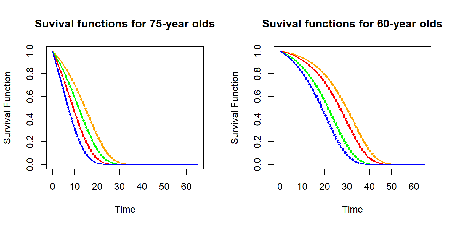
Figure 2.21: Survival functions for age 75 and different genders and smoking status (left), and survival curves for for 60-year old feamess with different BMI and blood pressure levels (right)

The survival functions are shown including 95% confidence intervals. As is evident, the covariates substantially affect the survival functions. Indeed, while 75-year old females have better survival prospects than males (orange vs. green curve on the left-hand side), female smokers are worse off than male non-smokers (green vs. red curve on the left-hand side) – while male smokers have the bleakest survival prospects (blue curve on the left-hand side). Similarly, for the 60-year old females, individuals with the low BMI and low blood pressure with a median future lifetime of more than 30 years (orange curve on the right-hand side), whereas for the highest levels of BMI (40) and systolic blood pressure (180), the median future lifetime is less than 20 years (blue curve on the right-hand side). We notice the inframarginal decrease in the survival probabilities as the BMI exceeds 30.

2.6.3 Conditional Life Tables

Recall that a life table is a discretized version of the survival function. Therefore, we can rely on the estimated survival function to generate a life table. We consider the example of a newly underwritten life in the month after the end of our dataset, for a 42-year-old non-smoking male with a BMI of 28 and a blood pressure of 127. We consider the discretized version of the survival function and determine annualized mortality probabilities \(q_{x+t}\), according to the formulas provides in Section 2.2.

R Code For Figure

par(mfrow=c(1,1))
s <- Survfunction(781,42,1,0,28,127)
S_x_t <- summary(s,times = 0:68)$surv
q_x_t <- rep(0,64)
for(i in 1:64){
  q_x_t[i] <- (S_x_t[i] - S_x_t[i+1])/S_x_t[i] 
}
plot(q_x_t,main="Mortality probabilities for 42 + t", xlab="t", ylab="q_x+t")
lines(q_x_t, lwd = 2, col = "blue")
xs <- 1:64
q_x_t_smoothed <- predict(loess(q_x_t~xs))
lines(q_x_t_smoothed, lwd = 2, col = "red")

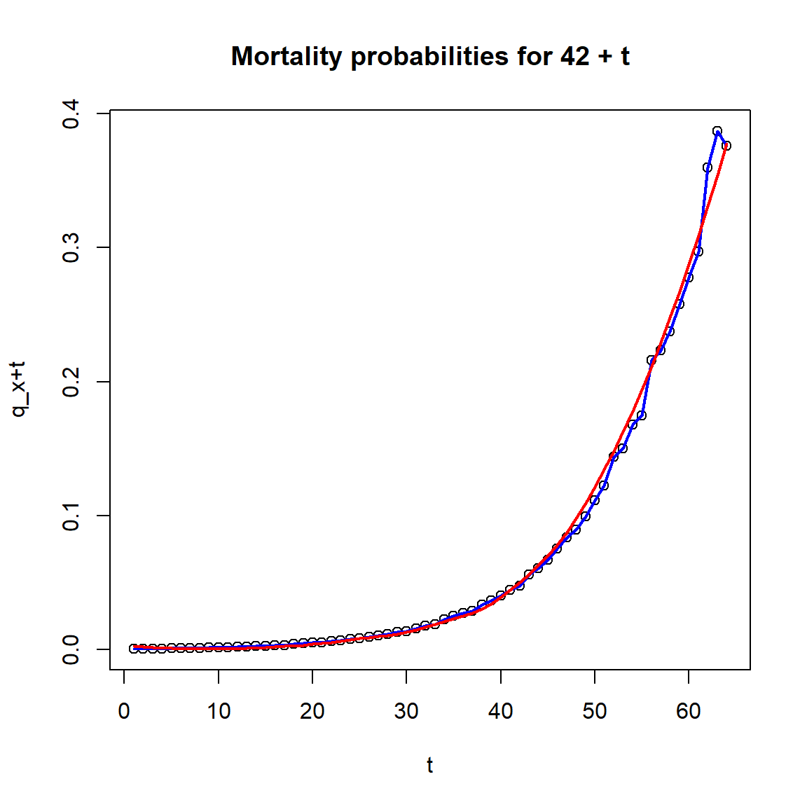
Figure 2.22: Mortality probabilities for a 42-year-old non-smoking male with a BMI of 28 and a blood pressure of 127.

We notice that the raw mortality probabilities (dots and blue curve) show some irregularities, so we also prvovide a smoothed version based on a local regression fit (via loess). The survival function and the mortality probabilities can be used for actuarial calculations.

Life insurance policies have a complex benefit structure that requires knowledge upon the probability of paying the benefits besides many other risk modeling parameters. Policy pricing, meeting the regulatory requirements, and understanding the life portfolio risk performance are all actuarial evaluations that rely on these risk modeling parameters. Mortality risk plays an important role for all of these. In the coming chapters, we discuss how – given (an estimate of) the distribution of the future lifetime random variable \(T_{\bf{x}}\) – we can perform these evaluations. In principle, any model discussed in this chapter can be used.

As we have seen, models of different degrees of sophistication are possible. What approach is adequate depends on the application in view. For instance, for statutory calculations governed by insurance regulation, often certain life tables are mandated that only account for a limited set of factors (sex, smoking status, etc.). In contrast, when pricing term life insurance policies, the underwriting process can be intricate and resulting information can be leveraged to quote a premium that closely reflects the adopted risk.

2.7 Notes and Comments

Reference to Survival analysis textbooks