Chapter 9 Bayesian Statistics and Modeling

Chapter Preview. Up to this point in the book, we have focused almost exclusively on the frequentistType of statistical inference based in frequentist probability, which treats probability in equivalent terms to frequency and draws conclusions from sample-data by means of emphasizing the frequency or proportion of findings in the data. approach to estimate our various loss distribution parameters. In this chapter, we switch gears and discuss a different paradigm: Bayesianism. These approaches are different as BayesianA type of statistical inference in which the model parameters and the data are random variables. and frequentist statisticians disagree on the source of the uncertainty: Bayesian statistics assumes that the observed data sample is fixed and that model parameters are random, whereas frequentism considers the opposite (i.e., the sample data are random, and the model parameters are fixed but unknown).

In this chapter, we introduce Bayesian statistics and modeling with a particular focus on loss data analytics. We begin in Section 9.1 by explaining the basics of Bayesian statistics: we compare it to frequentism and provide some historical context for the paradigm. We also introduce the seminal Bayes’ rule that serves as a key component in Bayesian statistics. Then, building on this, we present the main ingredients of Bayesian statistics in Section 9.2: the posterior distribution, the likelihood function, and the prior distribution. Section 9.3 provides some examples of simple cases where the prior distribution is chosen for algebraic convenience, giving rise to a closed-form expression for the posterior; these are called conjugate families in the literature. Section 9.4 is dedicated to cases where we cannot get closed-form expressions and for which numerical integration is needed. Specifically, we discuss two influential Markov chain Monte Carlo samplers: the Gibbs sampler and the Metropolis–Hastings algorithm. We also discuss how to interpret the chains obtained by these methods (i.e., Markov chain diagnostics). Finally, the last section of this chapter, Section 9.5, explains the main computing resources available and gives an illustration in the context of loss data.

9.1 A Gentle Introduction to Bayesian Statistics

In Section 9.1, you learn how to:

Describe qualitatively Bayesianism as an alternative to the frequentist approach.
Give the historical context for Bayesian statistics.
Use Bayes’ rule to find conditional probabilities.
Understand the basics of Bayesian statistics.

9.1.1 Bayesian versus Frequentist Statistics

Classic frequentist statistics rely on frequentist probability—an interpretation of probability in which an event’s probability is defined as the limit of its relative frequency (or propensity) in many, repeatable trials. It draws conclusion from a sample that is one of many hypothetical datasets that could have been collected; the uncertainty is therefore due to the sampling error associated with the sample, while model parameters and various quantities of interest are fixed (but unknown to the experimenter).

Example 9.1.1. Coin Toss. Considering the simple case of coin tossing, if we flip a fair coin many times, we expect to see heads about 50% of the time. If we flip the coin only a few times, however, we could see a different sample just by chance. Indeed, there is a non-zero probability of observing all heads (and this even if the sample is very large). Figure 9.1 illustrates this the number of heads observed in 100 samples of five iid tosses; in this specific example, we observe six samples for which all tosses are heads.⁹

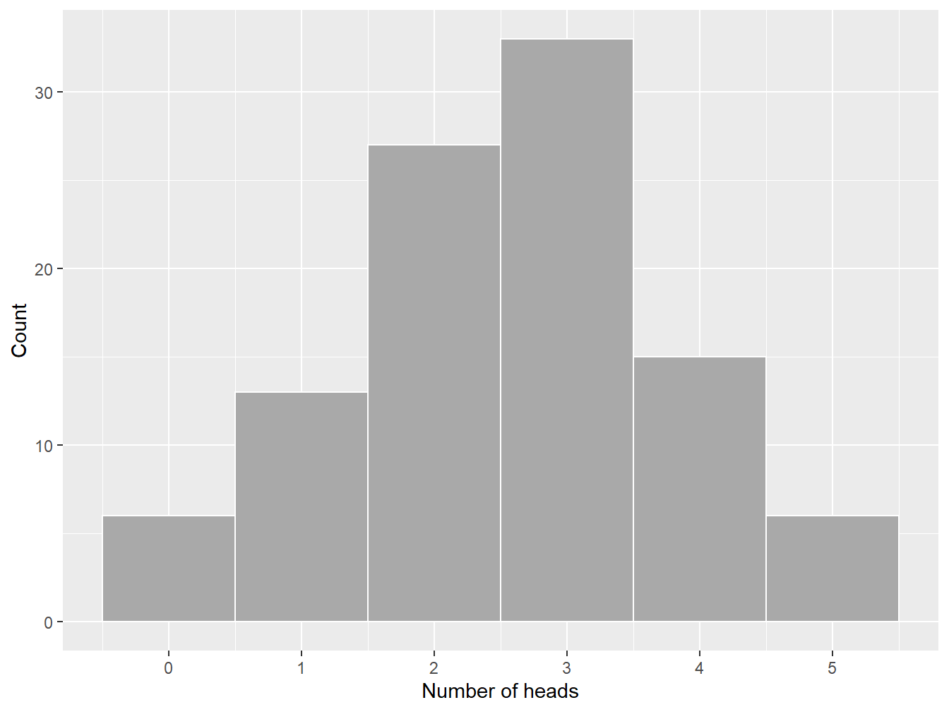
Figure 9.1: Frequency histogram of the number of heads in a sample of five data points

Yet, as the sample size increases, the relative frequency of heads should get closer to 50% if the coin is fair. Figure 9.2 reports that, if the number of tosses increases, then relative frequency of heads gets closer to 0.5—the probability of seeing heads on a given coin toss. In other words, increasing the sample size makes the resulting parameter estimate less uncertain, and the experimenter should be reaching a probability of 0.5 in the limit, assuming they can reproduce the experiment an infinite number of times.

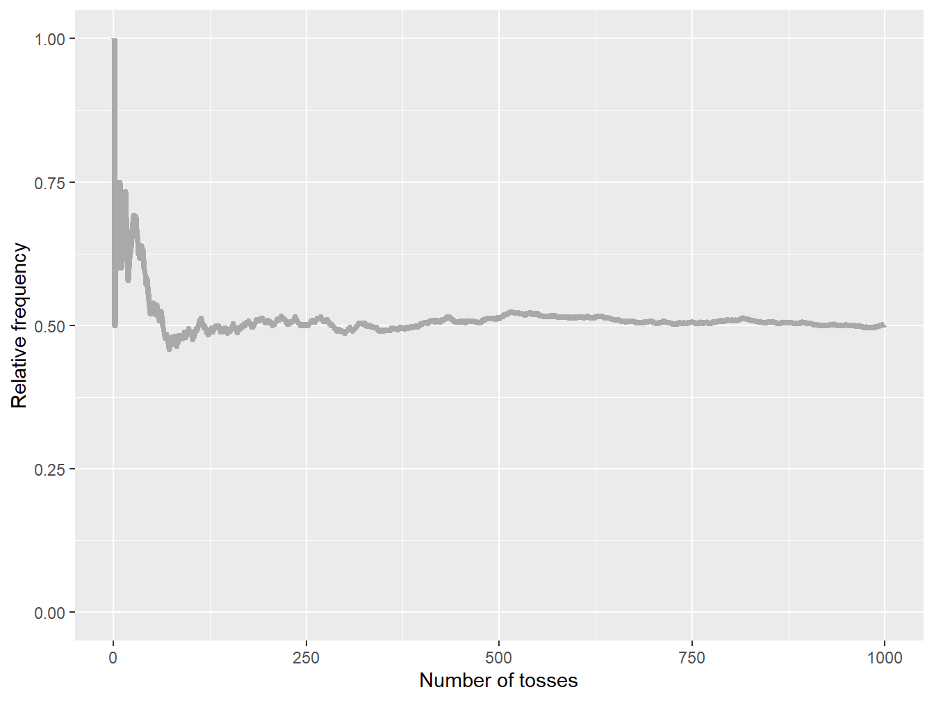
Figure 9.2: Cumulative relative frequencies of heads for an increasing sample size

Bayesians see things differently: they interpret probabilities as degrees of certainty about some quantity of interest. To find such probabilities, they draw on prior knowledge about those quantities, expressing one’s beliefs before some data are taken into account. Then, as data are collected, knowledge about the world is updated, allowing us to incorporate such new information in a consistent manner; the resulting distribution is referred to as the posterior, which summarizes the information in both the prior and the data.

In the context of Bayesian statistics and modeling, this interpretation of probability implies that model parameters are assumed to be random variables—unlike the frequentist approach that considers them fixed. Starting from the prior distribution, the data—summarized via the likelihood function—are used to update the prior distribution and create a posterior distribution of the parameters (see Section 9.2 for more details on the posterior distributionThe posterior distribution is the updated probability distribution of a parameter after incorporating prior information and observed data through Bayesian inference., the likelihood functionA function of the likeliness of the parameters in a model, given the observed data., and the prior distributionA probability distribution assigned prior to observing additional data). The influence of the prior distribution on the posterior distribution becomes weaker as the size of the observed data sample increases: the prior information is less and less relevant as new information comes in.

Example 9.1.1. Coin Toss, continued. We now reconsider the coin tossing experiment above through a Bayesian lens. Let us first assume that we have a (potentially unfair) coin, and we wish to understand the probability of obtaining heads, denoted by $q$ in this example. Consistent with the Bayesian paradigm, this parameter is random; let us assume that the random variable associated with the probability of observing heads is denoted by $Q$. For simplicity, we assume that we do not have prior information on the specific coin under investigation.¹⁰ Assuming again that our sample contains only five iid tosses, we know that the probability of observing $x$ heads is given by the binomial distribution with $m=5$ such that

\[ p_{X|Q=q}(x) = \mathrm{Pr}(X = x \, | \, Q = q) = \binom{5}{x} q^x (1-q)^{5-x}, \quad x \in \{0,1,...,5\}, \] where $0 \leq q \leq 1$, which emphasizes the fact that this probability depends on parameter $q$ by explicitly conditioning on it (unlike the notation used so far in this book, note that we append subscripts to the various pdf and pmf in this chapter to denote the random variables under study; this additional notation allows us to consider the pdf and pmf of different random variables in the same problem).

Let us generate a sample of these five tosses:

set.seed(1)
nbheads <- c(1)
num_flips <- 5
coin <- c("heads", "tails")
flips <- sample(coin, size = 5, replace = TRUE)
nbheads <- sum(flips == "heads")
cat("Number of heads:", nbheads)

Number of heads: 3

Based on this simulation, we obtain a data sample that contains three heads and two tails. Therefore, using Bayesian statistics, we can show that

\[ f_{Q|X=3}(q) \, \propto \, q^3 (1-q)^{2}, \] where $\propto$ means proportional to (note that obtaining this equation requires some tools that will be introduced in Section 9.2).¹¹ Figure 9.3 illustrates this pdf and reports the uncertainty about parameter $q$ based on this sample of five data points. In this example, one can see that the uncertainty is quite large; this is a by-product of using only five data points. Indeed, based on these five observations, one could argue that the probability should be close to $\frac{3}{5}=0.6$. This Bayesian analysis shows that 0.6 is likely, but that it is also very uncertain—a conclusion that is not direct in the frequentist approach.

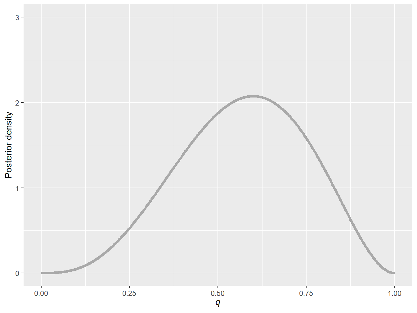
$Posterior probability density function of parameter $q$ for a sample of five data points$

Figure 9.3: Posterior probability density function of parameter $q$ for a sample of five data points

Figure 9.4, which is animated, reports the analog of Figure 9.2 through a Bayesian lens: we see the evolution of the posterior density of parameter $q$ as a function of the sample size for the same sample used in Figure 9.2. As we obtain more evidence, the posterior density becomes more concentrated around 0.5—a consequence of using a fair coin in the simulations above. Yet, even if the sample size if 1,000, we still see some parameter uncertainty.

$Posterior probability density function of parameter $q$ as a function of the sample size$

Figure 9.4: Posterior probability density function of parameter $q$ as a function of the sample size

But why be Bayesian? There are indeed several advantages to the Bayesian approach. First, this approach allows us to describe the entire distribution of parameters conditional on the data and to provide probability statements regarding the parameters that could be interpreted as such. Second, it provides a unified approach for estimating parameters. Some non-Bayesian methods, such as least squaresA technique for estimating parameters in linear regression. it is a standard approach in regression analysis to the approximate solution of overdetermined systems. in this technique, one determines the parameters that minimize the sum of squared differences between each observation and the corresponding linear combination of explanatory variables., require a separate approach to estimate variance components. In contrast, in Bayesian methods, all parameters can be treated in a similar fashion. Third, it allows experimenters to blend prior information from other sources with the data in a coherent manner.¹²

Are there any disadvantages to being Bayesian? Well, of course: while the Bayesian approach has many advantages, it is not without its disadvantages. First, it tends to be very computationally demanding (i.e., Bayesian methods often require complex computations, especially when dealing with high-dimensional problems or large datasets). For instance, complex models may not have closed-form solutions and require specialized computational techniques, which can be time-consuming. Second, there is some subjectivity in selecting priors—our initial beliefs and knowledge about the parameters—and this can lead to different results in the end. Third, Bayesian analysis often produces results that can be challenging to communicate effectively to non-experts.

Despite these disadvantages, the Bayesian approach remains powerful and flexible for many actuarial problems.

Do I need to be a Bayesian to embrace Bayesian statistics? No, this can be decided on a case-by-case basis. Consider a Bayesian study when you have prior knowledge or beliefs about the parameters, need to explicitly quantify uncertainty in your estimates, have limited data, require a flexible framework for complex models, or when decision-making under uncertainty is a key aspect of your analysis.

Even if one does not want to be a Bayesian truly, they can still recognize the usefulness of some of the methods. Indeed, some modern statistical tools in artificial intelligence and machine learning rely heavily on Bayesian techniques (e.g., Bayesian neural networks, Gaussian processes, and Bayesian classifiers, to name a few).

9.1.2 A Brief History Lesson

Interestingly, some have argued that the birth of Bayesian statistics is intimately related to insurance; see, for instance, Cowles (2013). Specifically, the Great Fire of London in 1666—destroying more than 10,000 homes and about 100 churches—led to the rise of insurance as we know it today. Shortly after, the first full-fledged fire insurance company came into existence in England during the 1680s. By the turn of the century, the idea of insurance was well ingrained and its use was booming in England; see, for instance, Haueter (2017). Yet, the lack of statistical models and methods—much needed to understand risk—drove some insurers to bankruptcy.

Thomas Bayes, an English statistician, philosopher and Presbyterian minister, applied his mind to some of these important statistical questions raised by insurers. This culminated into Bayes’ theory of probability in his seminal essay entitled Essay towards solving a problem in the doctrine of chances, published posthumously in 1763. This essay laid out the foundation of what we now know as Bayesian statistics.

Figure 9.5: Portrait of an unknown Presbyterian clergyman identified as Thomas Bayes in O’Donnell (1936)

Thomas Bayes’ work also helped Pierre-Simon Laplace, a famous French scholar and polymath, to develop and popularize the Bayesian interpretation of probability in the late 1700s and early 1800s. He also moved beyond Bayes’ essay and generalized his framework. Laplace’s efforts were followed by many, and Bayesian thinking continued to progress throughout the years with the help of statisticians like Bruno de Finetti, Harold Jeffreys, Dennis Lindley, and Leonard Jimmie Savage.

Nowadays, Bayesian statistics and modeling is widely used in science, thanks to the increase in computational power over the past 30 years. Actuarial science and loss modeling, more specifically, have also been breeding grounds for Bayesian methodology. So, Bayesian statistics circles back to insurance, in a sense, where it all started.

9.1.3 Bayes’ Rule

This subsection introduces how the Bayes’ rule is applied to calculating conditional probabilities for events.

Conditional Probability. The concept of conditional probability considers the relationship between probabilities of two (or more) events happening. In its most simple form, being interested in conditional probability boils down to answering this question: given that event $B$ happened, how does this affect the probability that $A$ happens? To answer this question, we can define formally the concept of conditional probability:

\[ \Pr\left(A \, \middle| \, B\right) = \frac{\Pr(A \cap B)}{\Pr(B)}. \] To be properly defined, we must assume that $\Pr(B)$ is larger than zero; that is, event $B$ is not impossible. Simply put, a conditional probability turns $B$ into the new probability space, and then cares only about the part of $A$ that is inside $B$ (i.e., $A \cap B$).

Example 9.1.2. Actuarial Exam Question. An insurance company estimates that 40% of policyholders who have an extended health policy but no long-term disability policy will renew next year, and 70% of policyholders who have a long-term disability policy but no extended health policy will renew next year. The company also estimates that 50% of their clients who have both policies will renew at least one next year. The company records report that 65% of clients have an extended health policy, 40% have a long-term disability policy, and 10% have both. Using the data above, calculate the percentage of policyholders that will renew at least one policy next year.¹³

Show Example Solution

Independence. If two events are unrelated to one another, we say that they are independentTwo variables are independent if conditional information given about one variable provides no information regarding the other variable. Specifically, $A$ and $B$ are independent if

\[ \Pr(A \cap B) = \Pr(A) \, \Pr(B). \] For positive probability events, independence between $A$ and $B$ is also equivalent to

\[ \Pr(A\,|\, B) = \Pr(A) \quad \text{and} \quad \Pr(B\,|\, A) = \Pr(B), \] which means that the occurrence of event $B$ does not have an impact on the occurrence of $A$, and vice versa.

Bayes’ Rule. Intuitively speaking, Bayes’ rule provides a mechanism to put our Bayesian thinking into practice. It allows us to update our information by combining the data—from the likelihood—and the prior together to obtain a posterior probability.

Proposition 9.1.1. Bayes’ Rule for Events. For events $A$ and $B$, the posterior probability of event $A$ given $B$ follows

\[ \Pr(A\,|\,B) = \frac{\Pr(B\, |\, A) \Pr(A)}{\Pr(B)}, \] where the law of total probability allows us to find

\[ \Pr(B) = \Pr(A) \Pr(B \, | \, A) + \Pr(A^{\text{c}}) \Pr(B \, |\, A^{\text{c}}). \] Note, again, that this works as long as event $B$ is possible (i.e., $\Pr(B) > 0$).¹⁴

Show A Snippet of Theory

Simply put, the posterior probability of event $A$ given $B$ is obtained by combining the likelihood of $B$ given a fixed $A$—proxied by $\Pr(B\, |\, A)$—with the prior probability of observing $A$, and then dividing it by the marginal probability of event $B$ to make sure that the probabilities sum up to one.

Example 9.1.3. Actuarial Exam Question. An automobile insurance company insures drivers of all ages. An actuary compiled the probability of having an accident for some age bands as well as an estimate of the portion of the company’s insured drivers in each age band:

\[ \begin{matrix} \begin{array}{c|c|c} \hline \text{Age of Driver} & \text{Probability of Accident} & \text{Portion of Company's } \\ & & \text{Insured Drivers} \\\hline \text{16-20} & 0.06 & 0.08 \\\hline \text{21-30} & 0.03 & 0.15 \\\hline \text{31-65} & 0.02 & 0.49 \\\hline \text{66-99} & 0.04 & 0.28 \\\hline \end{array} \end{matrix} \]

A randomly selected driver that the company insures has an accident. Calculate the probability that the driver was age 16-20.¹⁵

Show Example Solution

9.1.4 An Introductory Example of Bayes’ Rule

The example above illustrates how to use Bayes’ rule in an academic context; the focus of this book is, nonetheless, data analytics. We therefore also wish to illustrate Bayes’ rule by using real data. In this introductory example, we use the Singapore auto data sgautonb of the R package CASdatasets that was already used in Chapter 3.

library("CASdatasets")
data(sgautonb)

This dataset contains information about the number of car accidents and some risk factors (i.e., the type of the vehicle insured, the age of the vehicle, the sex of the policyholder, and the age of the policyholder grouped into seven categories).¹⁶

Example 9.1.4. Singapore Insurance Data. A new insurance company—targeting an older segment of the population—estimates that 20% of their policyholders will be 65 years old and older. The actuaries working at the insurance company believes that the Singapore insurance dataset is credible to understand the accident occurrence of the new company. Based on this information, find the probability that a randomly selected driver who has (at least) one accident, is 65 years or older.

Show Example Solution

Solution. Let $O$ denote the event related to the policyholder being 65 years old and older (i.e., Age Category 6 in the dataset), and $A$ the event of a policyholder having at least an accident. Using Bayes’ rule, we have that

\[ \Pr(O\, |\, A) = \frac{\Pr(A\, |\, O)\Pr(O)}{\Pr(A)}, \]

where the prior probability $\Pr(O)$ is given by the problem statement: $\Pr(O) = 0.20$. This implies that $\Pr(O^{\text{c}}) = 1-0.20 = 0.80$. From the Singapore insurance data, we know that $\Pr(A\, |\, O) = 0.1082803$ and $\Pr(A\, |\, O^{\text{c}}) = 0.06415506$, which allow us to use the law of total probability to obtain:

\[ \Pr(A) = \Pr(A\, |\, O)\Pr(O) + \Pr(A\, |\, O^{\text{c}})\Pr(O^{\text{c}}). \]

n <- length(sgautonb$AgeCat)
nO <- sum(sgautonb$AgeCat == 6)
nOc <- sum(sgautonb$AgeCat != 6)
nAandO <- sum(sgautonb$AgeCat == 6 & sgautonb$Clm_Count > 0)
nAandOc <- sum(sgautonb$AgeCat != 6 & sgautonb$Clm_Count > 0)

PAO <- nAandO/nO
PAOc <- nAandOc/nOc

POA <- PAO * 0.2/(PAO * 0.2 + PAOc * 0.8)
cat("The probability that policyholder having accident is 65 years old and older is",
    POA)

The probability that policyholder having accident is 65 years old and older is 0.296739115

The probability that a randomly selected driver who has (at least) one accident, is 65 years or older is therefore about 29.7% for the new insurance company. Simply put, we started with an a priori probability of 20%, meaning that unconditionally, we should have about 20% of policyholders aged 65 years old and older, and that 20% of the policyholders should have at least one accident. Then, based on the observed data, this probability is updated to 29.7%: the data seem to imply that, of all people having accidents, there are more older policyholders than what we would have guessed just based on our prior assumption.

In the next section, we expand on the idea of Bayes’ rule and apply it to slightly more general cases involving random variables instead of events.

9.2 Building Blocks of Bayesian Statistics

In Section 9.2, you learn how to:

Describe the main components of Bayesian statistics; that is, the posterior distribution, the likelihood function, and the prior distribution.
Summarize the different classes of priors used in practice.

Proposition 9.1.1 above deals with the elementary case of Bayes’ rule for events. Although this version of Bayes’ rule is useful to understand the foundation of Bayesian statistics, we will need slightly more general versions of it to achieve our aim. Specifically, Proposition 9.1.1 needs to be generalized to the case of random variables.

Let us first consider the case of discrete random variables. Assume $X$ and $Y$ are both discrete random variables that allow for the following joint pmf of

\[ p_{X,Y}(x,y) = \Pr(X=x \,\text{ and }\, Y=y) \]

as well as the following marginal distributions for $X$ and $Y$:

\[ p_X(x)= \Pr(X=x) = \sum_k p_{X,Y}(x,k) \quad \text{and} \quad p_Y(y)= \Pr(Y=y) = \sum_k p_{X,Y}(k,y), \]

respectively. Using the result of Proposition 9.1.1 and setting event $A$ as $\{Y=y\}$ and $B$ as $\{X=x\}$ yields

\[ p_{Y|X=x}(y)= \frac{p_{X|Y=y}(x)\, p_Y(y)}{p_X(x)}, \]

where $p_{Y|X=x}(y) = \Pr\left( Y = y \, \middle|\, X = x\right)$ is the conditional pmf of $Y$ conditional on $X$ being equal to $x$. Using the law of total probability,

\[ p_X(x)= \sum_k p_{X,Y}(x,k) = \sum_k p_{X|Y=k}(x) \, p_Y(k), \]

we can rewrite the denominator above to get the following version of Bayes’ rule:

\[ p_{Y|X=x}(y) = \frac{p_{X|Y=y}(x)\, p_Y(y)}{\sum_k p_{X|Y=k}(x) \, p_Y(k)}. \]

We can also obtain a similar Bayes’ rule for continuous random variables by replacing probability mass functions by probability density functions, and sums by integrals.

Proposition 9.2.1. Bayes’ Rule for Continuous Random Variables. For two continuous random variables $X$ and $Y$, the conditional probability density function of $Y$ given $X=x$ follows

\[ f_{Y|X=x}(y) = \frac{f_{X|Y=y}(x)\, f_Y(y)}{f_X(x)}, \]

where the marginal distributions of $X$ and $Y$ are given as follows:

\[ f_X(x)=\int_{-\infty}^{\infty} \! f_{X,Y}(x,u) \, du \quad \text{and} \quad f_Y(y)=\int_{-\infty}^{\infty} \! f_{X,Y}(u,y) \, du, \]

respectively. Similar to the discrete random variable case, we can swap the denominator of the equation above for

\[ f_{X}(x) = \int_{-\infty}^{\infty} \! f_{X,Y}(x,u) \, du = \int_{-\infty}^{\infty} \! f_{X|Y=u}(x) \, f_Y (u) \, du \]

by using the law of total probability.

Show A Snippet of Theory

Note that one can mix the discrete and continuous definitions of Bayes’ rule to accommodate for cases where the parameters have continuous random variables and the observations are expressed via discrete random variables, or vice versa.

9.2.1 Posterior Distribution

Model parameters are assumed to be random variables under the Bayesian paradigm, meaning that Bayes’ rule for (discrete or continuous) random variables can be applied to update the prior knowledge about parameters by using new data. This is indeed similar to the process used in Section 9.1.1.

Let us consider only one unknown model parameter $\theta$ associated with random variable $\Theta$ for now.¹⁷ Further, consider $n$ observations

\[ \mathbf{x} = (x_1, x_2, ..., x_n), \]

which are realizations of the collection of random variables

\[ \mathbf{X} = (X_1, X_2, ..., X_n). \]

If $Y$ in Proposition 9.2.1 is replaced by $\Theta$ and $X$ by $\mathbf{X}$, we obtain

\[ f_{\Theta|\mathbf{X}=\mathbf{x}}(\theta) = \frac{f_{\mathbf{X}|\Theta=\theta}(\mathbf{x})\, f_{\Theta}(\theta)}{f_{\mathbf{X}}(\mathbf{x})}, \]

which represents the posterior distribution of the model parameter after updating the distribution based on the new observations $\mathbf{x}$, and where

$f_{\mathbf{X}|\Theta=\theta}(\mathbf{x})$ is the likelihood function, also known as the conditional joint pdf of the observations assuming a given value of parameter $\theta$,
$f_{\Theta}(\theta)$ is the unconditional pdf of the parameter that represents the prior information, and
$f_{\mathbf{X}}(\mathbf{x})$ is the marginal likelihood, which is a constant term with respect to $\theta$, making the posterior density integrate to one.

In other words, Bayes’ rule provides a way to update the prior distribution of the parameter into a posterior distribution—by considering the observations $\mathbf{x}$.

Note that the marginal likelihood is constant once we have the observations. It does not depend on $\theta$ and does not impact the overall shape of the pdf: it only provides the adequate scaling to ensure that the density integrates to one. For this reason, it is common to write down the posterior distribution using a proportional relationship instead:

\[ f_{\Theta|\mathbf{X}=\mathbf{x}}(\theta) \propto \underbrace{f_{\mathbf{X}|\Theta=\theta}(\mathbf{x})}_{\text{Likelihood}} \, \, \underbrace{\vphantom{f_{\mathbf{X}|\Theta=\theta}(\mathbf{x})}f_{\Theta}(\theta)}_{\text{Prior}}. \]

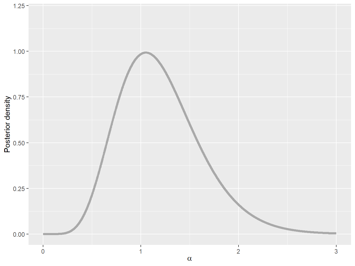
Example 9.2.1. A Problem Inspired from Meyers (1994). A car insurance pays the following (independent) claim amounts on an automobile insurance policy:

\[ 1050, \quad\quad 1250, \quad\quad 1550, \quad\quad 2600, \quad\quad 5350, \quad\quad 10200. \]

The amount of a single payment is distributed as a single-parameter Pareto distribution with $\theta = 1000$ and $\alpha$ unknown, such that

\[ f_{X_i|A=\alpha}(x_i) = \frac{\alpha \, 1000^{\alpha}}{x_i^{\alpha+1}}, \quad x_i \in \mathbb{R}_+. \]

We assume that the prior distribution of $\alpha$ is given by a gamma distribution with shape parameter 2 and scale parameter 1, and its pdf is given by

\[ f_{A}(\alpha) = \alpha\,e^{-\alpha}, \quad \alpha \in \mathbb{R}_+. \]

Find the posterior distribution of parameter $\alpha$.

Show Example Solution

The discussion above considered continuous random variables, but the same logic can be applied to discrete random variables by replacing probability density functions by probability mass functions.

Example 9.2.2. Coin Toss Revisited. Assume that you observe three heads out of five (independent) tosses. Each toss has a probability of $q$ of observing heads and $1-q$ of observing tails. Find the posterior distribution of $q$ assuming a uniform prior distribution over the interval $[0,1]$.

Show Example Solution

In the following subsections, we will discuss at greater length the two main building blocks used to build the posterior distribution: the likelihood function and the prior distribution.

9.2.2 Likelihood Function

The likelihood function is a fundamental concept in statistics. It is used to estimate the parameters of a statistical model based on observed data. As mentioned in previous chapters, the likelihood function can be used to find the maximum likelihood estimator. In Bayesian statistics, the likelihood function is used to update the prior based on the evidence (or data).

As explained above and in Chapter 17, the likelihood function is defined as the conditional joint pdf or pmf of the observed data, given the model parameters. In other words, it is the probability of observing the data given a specific parameter values.

Mathematically, the likelihood function is written as $f_{\mathbf{X}|\Theta=\theta}(x)$ (for continuous random variables) or $p_{\mathbf{X}|\Theta=\theta}(x)$ (for discrete random variables). Note that, throughout the book, the notation $L(\theta|\mathbf{x})$ has also been used for the likelihood function, and we will use both interchangeably in this chapter.

Special Case: Independent and Identically Distributed Observations. Oftentimes, in many problems and real-world applications, the observations are assumed to be iid. If they are, then we can easily write the likelihood function as:

\[ f_{\mathbf{X}|\Theta=\theta}(\mathbf{x}) = \prod_{i=1}^n f_{X_i|\Theta=\theta}(x_i) \quad \text{ or } \quad p_{\mathbf{X}|\Theta=\theta}(\mathbf{x}) = \prod_{i=1}^n p_{X_i|\Theta=\theta}(x_i). \]

9.2.3 Prior Distribution

In the Bayesian paradigm, the prior distribution represents our knowledge or beliefs about the unknown parameters before we observe any data. It is a probability distribution that expresses the uncertainty about the values of the parameters. The prior distribution is typically specified by choosing a family of probability distributions and selecting specific values for its parameters.

The choice of prior distribution is subjective and often based on external information or previous studies. In some cases, noninformative priors can be used, which represent minimal prior knowledge or assumptions about the parameters. In other cases, informative and weakly informative priors can be used, which incorporate prior knowledge or assumptions based on external sources. The selection of the prior distribution should be carefully considered, and sensitivity analysis can be performed to assess the robustness of the results to different prior assumptions.

Why Does It Matter? The choice of prior distribution can have a significant impact on the results of a Bayesian analysis. Different prior distributions can lead to different posterior distributions, which are the updated probability distributions for the parameters after we observe the data. Therefore, it is important to choose a prior distribution that reflects our prior knowledge or beliefs about the parameters.

9.2.3.1 Informative and Weakly Informative Priors

InformativeAn informative prior, in statistics, is a prior probability distribution that is chosen deliberately to incorporate specific information or beliefs about a parameter before observing new data. and weakly informativeA weakly informative prior is a prior probability distribution that introduces some general constraints or vague beliefs about a parameter, without heavily influencing the final inference. priors are terms used to describe the amount of prior knowledge or beliefs that is incorporated into a statistical model. Informative priors contain substantial prior knowledge about the parameters of a model, while weakly informative priors contain moderate prior knowledge.

Informative priors are useful when there is strong, potentially subjective prior information available about the model parameters, which can help to constrain the posterior distribution and improve inference. For example, in an insurance claims analysis study, an informative prior may be used to incorporate previous knowledge, such as the results of a previous claims study.

On the other hand, weakly informative priors are used when there is some—yet little—prior knowledge available or when the goal is to allow the data to drive the analysis. Weakly informative priors are designed to mildly impact the posterior distribution and are often chosen based on principles such as symmetry or scale invariance.

Overall, the choice of prior depends on the specific problem at hand and the available prior knowledge or beliefs. Informative priors can be useful when prior information is available and can improve the precision of the posterior distribution. In contrast, weakly informative priors can be useful when the goal is to allow the data to drive the analysis and avoid imposing strong prior assumptions.

Example 9.2.3. Actuarial Exam Question. You are given:

Annual claim frequencies follow a Poisson distribution with mean $\lambda$.
The prior distribution of $\lambda$ has the following pdf: \[ f_{\Lambda}(\lambda) = (0.3) \frac{1}{6} e^{-\frac{\lambda}{6}} + (0.7) \frac{1}{12} e^{-\frac{\lambda}{12}}, \quad \text{where } \lambda > 0. \]

Ten claims are observed for an insured in Year 1. Calculate the expected value of the posterior distribution of $\lambda$.¹⁸

Show Example Solution

9.2.3.2 Noninformative Priors

It is possible to take the idea of weakly informative priors to the extreme by using noninformativeA noninformative prior is a prior probability distribution that intentionally avoids incorporating specific information or strong beliefs about a parameter. priors. A noninformative prior is a prior distribution that is intentionally chosen to allow the data to have a more decisive influence on the posterior distribution rather than being overly influenced by prior beliefs or assumptions.

Noninformative priors can take different forms, such as flat priors, for instance. A flat prior assigns equal probability to all possible parameter values without additional information or assumptions.

Example 9.2.4. Informative Versus Noninformative Priors. You wish to investigate the impact of having informative and noninformative priors on a claim frequency analysis. Assume that the claim frequency for each policy follows a Bernoulli random variable with a probability of $q$ such that

\[ q_{X_i|Q=q}(x_i) = q^{x_i} (1-q)^{1-x_i}, \quad x_i \in \{0,1\}, \]

where $q \in [0,1]$, and consider two different prior distributions:

Informative: Based on past experience, you know that the claim probability is typically less than 5%, thus justifying the use of a uniform distribution over $[0,0.05]$.
Noninformative: You do not wish your posterior distribution to be impacted by your prior assumption and simply select a uniform distribution over the domain of $q$, which is $[0,1]$.

Using the first 100 lines of the Singapore insurance dataset (see Example 9.1.4 for more details on this dataset), find the two posterior distributions as well as the posterior expected value of the probability $q$ under both prior assumptions.

Show Example Solution

Solution. Let us start with the informative prior, where

\[ f_Q(q)= \frac{1}{0.05 - 0} = 20, \quad \text{ if }\, q \in [0, 0.05], \]

and zero otherwise. In this case, assuming $x = \sum_{i=1}^{100} x_i$, the posterior density is given by

\[\begin{align} f_{Q|\mathbf{X}=\mathbf{x}} (q) \propto &\, f_{\mathbf{X}|Q=q}(\mathbf{x}) f_Q(q) \\ \propto& \, \prod_{i=1}^{100} q^{x_i} (1-q)^{1-x_i} \\ = &\, q^{x} (1-q)^{100-x}, \quad \text{ if }\, 0 \leq q \leq 0.05, \end{align}\]

and zero otherwise. We can numerically obtain the shape of this posterior distribution by dividing $q^{x} (1-q)^{100-x}$ by

\[ \int_0^{0.05} \! q^{x} (1-q)^{100-x} \, dq. \]

Note that this prior makes it impossible for the estimated frequency to be greater than 0.05.

The second prior is still uniform, but over $[0,1]$ this time, which is given mathematically by

\[ f_Q(q)= \frac{1}{1 - 0} = 1, \quad \text{ if }\, q \in [0,1], \]

and zero otherwise, leading to the following posterior distribution:

\[\begin{align} f_{Q|\mathbf{X}=\mathbf{x}} (q) \propto &\, f_{\mathbf{X}|Q=q}(\mathbf{x}) f_Q(q) \\ \propto & \, \prod_{i=1}^{100} q^{x_i} (1-q)^{1-x_i} \\ = &\, q^{x} (1-q)^{100-x}, \quad \text{ if }\, 0 \leq q \leq 1, \end{align}\]

and zero otherwise.

qs <- seq(from = 0, to = 0.12, by = 0.0001)
x <- sum(sgautonb$Clm_Count[1:100])

integrandposterior1 <- function(q) {
    q^x * (1 - q)^(100 - x) * ifelse(q >= 0 & q <= 0.05, 1, 0)
}
marglikelihood1 <- integrate(integrandposterior1, 0, 1, abs.tol = .Machine$double.eps^2)$value
posterior1 <- integrandposterior1(qs)/marglikelihood1

integrandposterior2 <- function(q) {
    q^x * (1 - q)^(100 - x) * ifelse(q >= 0 & q <= 1, 1, 0)
}
marglikelihood2 <- integrate(integrandposterior2, 0, 1, abs.tol = .Machine$double.eps^2)$value
posterior2 <- integrandposterior2(qs)/marglikelihood2

Figure 9.7: Posterior densities based on informative (gray) and noninformative priors (black)

We also wish to obtain the expected value of $q$ for both posterior distribution. This can be obtained by numerically integrating the following equation:

\[ \mathrm{E}[Q|\mathbf{X}=\mathbf{x}] = \int_0^1 \! q \, f_{Q|\mathbf{X}=\mathbf{x}} (q) \, dq. \]

integrandexpvalue1 <- function(q) {
    integrandposterior1(q)/marglikelihood1 * q
}
expectedvalue1 <- integrate(integrandexpvalue1, 0, 1, abs.tol = .Machine$double.eps^2)$value
cat("The posterior expected value of the parameter when using the informative prior is",
    expectedvalue1)

The posterior expected value of the parameter when using the informative prior is 0.0304525117

integrandexpvalue2 <- function(q) {
    integrandposterior2(q)/marglikelihood2 * q
}
expectedvalue2 <- integrate(integrandexpvalue2, 0, 1, abs.tol = .Machine$double.eps^2)$value
cat("The posterior expected value of the parameter when using the noninformative prior is",
    expectedvalue2)

The posterior expected value of the parameter when using the noninformative prior is 0.0392156863

As one can see, these values are different, meaning that the prior distribution can have a material impact on the posterior distribution. One should therefore be careful when selecting a prior distribution.

9.2.3.3 Improper Priors

An improperAn improper prior is a prior probability distribution that does not integrate to a finite value over the entire parameter space. prior is a prior distribution that is not a proper probability distribution, meaning that it does not integrate (or sum) to one over the entire parameter space. Improper priors can be used in Bayesian analyses, but they require careful handling because they can lead to improper posterior distributions.

Improper priors are typically used when there is little or no prior information about the parameter of interest—some noninformative priors are indeed improper—and they can be thought of as representing a very diffuse or noncommittal prior belief. For instance, the uniform distribution on an infinite interval is a common choice of improper prior.

Example 9.2.5. Improper Prior, Proper Posterior. Let us assume a random sample $\mathbf{x}$ of size $n$, which is a realization of the collection of random variables $\mathbf{X} = (X_1,X_2, ..., X_n)$. Further, assume that each random variable $X_i$ is independent and normally distributed with mean of $\mu$ and variance of 1:

\[ f_{X_i|M=\mu}(x_i) = \frac{1}{\sqrt{2\pi}} \exp\left( - \frac{1}{2} \left( x_i -\mu\right)^2 \right), \quad x_i \in \mathbb{R}, \]

where $\mu$ is a (random) parameter. Obtain the posterior distribution of $\mu$ assuming that its prior distribution is improper and given by $f_M(\mu) \propto 1$, where $\mu \in \mathbb{R}$.

Show Example Solution

Special care is needed when dealing with improper priors. Indeed, if one can derive the posterior distribution in closed form and show that it is proper—like in Example 9.2.5—it should not be a concern. On the other hand, in cases where the posterior distribution cannot be obtained in closed form, there is no assurance that the posterior will be proper and extra attention is required.

9.2.3.4 Choice of the Prior Distribution

The selection of a prior in Bayesian statistics is a crucial step that reflects the experimenter’s prior beliefs, knowledge, or assumptions about the parameters of interest. There are different approaches to selecting priors.

Informative priors are generally based on the experimenter’s subjective beliefs, knowledge, or experience. For instance, one might have a subjective belief that a parameter is likely to fall within a certain range, and this belief is formalized as an informative prior distribution.
Noninformative priors are chosen to be minimally informative, expressing little or no prior information about the parameters. For example, uniform priors are commonly used as noninformative priors, expressing a lack of prior preference for any particular parameter value.
Empirical Bayes priors rely on the data itself, combining empirical information with Bayesian methodology. This can be done by estimating a prior distribution hyperparameter by using the observed data to inform the prior distribution.
Priors that rely on expert elicitation involves seeking input from domain experts to inform the prior. For instance, the experimenter might have additional knowledge about the problem at hand and use a prior distribution that represents their beliefs about the parameters.

9.2.3.5 Prior Sensitivity Analysis

Prior sensitivity analysis is an important step in Bayesian modeling processes. It refers to the examination and evaluation of the impact of different prior assumptions on the results of a statistical analysis. In other words, such analyses aim to verify the robustness of the conclusions drawn from Bayesian inference to the choice of the prior distribution. By exploring a range of plausible prior distributions, experimenters can gain insights into how much the choice of prior influences the final results and whether those conclusions remain consistent under different prior assumptions.

For instance, prior distributions may significantly influence the posterior estimates, leading to different conclusions. Some of these might be subjective (i.e., informative priors) or based on expert knowledge, and assessing the impact of such assumptions promotes transparency and objectivity in the analysis.

9.3 Conjugate Families

In Section 9.3, you learn how to:

Describe three specific classes of conjugate families.
Use conjugate distributions to determine posterior distributions of parameters.
Understand the pros and cons of conjugate family models.

In Bayesian statistics, if a posterior distribution comes from the same distribution as the prior distribution, the prior and posterior are called conjugate distributionsDistributions such that the posterior and the prior come from the same family of distributions.. Note that both posterior and prior have similar shapes but will have different parameters, generally speaking.

But Why? Two main reasons explain why conjugate families have been so popular historically:

They are easy to use from a computational standpoint: posterior distributions in most conjugate families can be obtained in closed form, making this class of models easy to use even if we do not have access to computing power.
They tend to be easy to interpret: posterior distributions are compromises between data and prior distributions. Having both prior and posterior distributions in the same family—but with different parameters—allows us to understand and quantify how the data changed our initial assumptions.

9.3.1 The Beta–Binomial Conjugate Family

The first conjugate family that we investigate in this book is the beta–binomial family. Let $\mathbf{X} = (X_1, X_2, ... X_m)$ represent a sample of iid Bernoulli random variables such that

\[ X_i = \begin{cases} 1 & \text{if success} \\ 0 & \text{if failure} \end{cases} , \]

with probabilities $q$ and $1-q$, respectively. Let us further define $x = \sum_{i=1}^m x_i$ the sum of the realized successes.

We know from elementary probability that $X = \sum_{i=1}^m X_i$ follows a binomial distribution (i.e., the number of successes $x$ in $m$ Bernoulli trials) with unknown probability of success $q$ in $[0,1]$, similar to the coin tossing case of Example 9.1.1, such that the likelihood function is given by

\[ p_{\mathbf{X}|Q=q}(\mathbf{x}) = \binom{m}{x} q^x (1-q)^{m-x}, \quad x \in \{0,1,...,m\}, \]

where $x = \sum_{i=1}^m x_i$. The latter represents our evidence. Then, we combine it with its usual conjugate prior—the beta distribution with parameters $a$ and $b$. The pdf of the beta distribution is given as follows:

\[ f_{Q}(q) = \frac{\Gamma(a+b)}{\Gamma(a)\Gamma(b)} q^{a-1} (1-q)^{b-1}, \quad q \in [0,1], \]

where $a$ and $b$ are shape parameters of the beta distribution.¹⁹

We can now combine the prior distribution—beta—with the likelihood function—binomial—to obtain the posterior distribution.

Proposition 9.3.1. Beta–Binomial Conjugate Family. Consider a sample of $m$ iid Bernoulli experiments $(X_1,X_2,...,X_m)$ each with success probability $q$. Further assume that the random variable associated with the success probability, $Q$, has a prior that is beta with shape parameters $a$ and $b$. The posterior distribution of $Q$ is therefore given by

\[ f_{Q|\mathbf{X}=\mathbf{x}}(q) = \frac{\Gamma(a+b+m)}{\Gamma(a+x)\Gamma(b+m-x)} q^{a+x-1} (1-q)^{b+m-x-1}, \]

where $x = \sum_{i=1}^m x_i$, which is a beta distribution with shape parameters $a+x$ and $b+m-x$.

Show A Snippet of Theory

Parameters Versus Hyperparameters. In this context, $a$ and $b$ are called hyperparametersHyperparameters are parameters that define the distribution of a prior distribution—parameters of the prior. These are different from parameters of the underlying model (i.e., $q$ in the beta–binomial family). Hyperparameters are typically assumed and determined by the experimenter, whereas the underlying model parameters are random in the Bayesian context.

Example 9.3.1. Actuarial Exam Question. You are given:

The annual number of claims in Year $i$ for a policyholder has a binomial distribution with pmf \[ p_{X_i|Q=q}(x_i) = \binom{2}{x} q^{x_i} (1-q)^{2-x_i}, \quad x_i \in \{ 0, 1, 2\}. \]
The prior distribution is

\[ f_Q(q) = 4 q^3, \quad q \in [0,1]. \]

The policyholder had one claim in each of Years 1 and 2. Calculate the Bayesian estimate of the expected number of claims in Year 3.²⁰

Show Example Solution

Example 9.3.2. Impact of Beta Prior on Posterior. You wish to investigate the impact of having different beta hyperparameters on the posterior distribution. Assume that the claim frequency for each policy follows a Bernoulli random variable with a probability of $q$ such that

\[ p_{X_i|Q=q}(x_i) = q^{x_i} (1-q)^{1-x_i}, \quad x_i \in \{0,1\}, \]

where $q \in [0,1]$, and consider two different sets of hyperparameters:

Set 1: $a = 1$ and $b=10$.
Set 2: $a = 2$ and $b=2$.

Figure 9.8 shows the pdf of these two prior distributions. The first prior assumes a small prior mean frequency of $\frac{1}{11}$, whereas the second prior distribution has a mean of $\frac{1}{2}$.

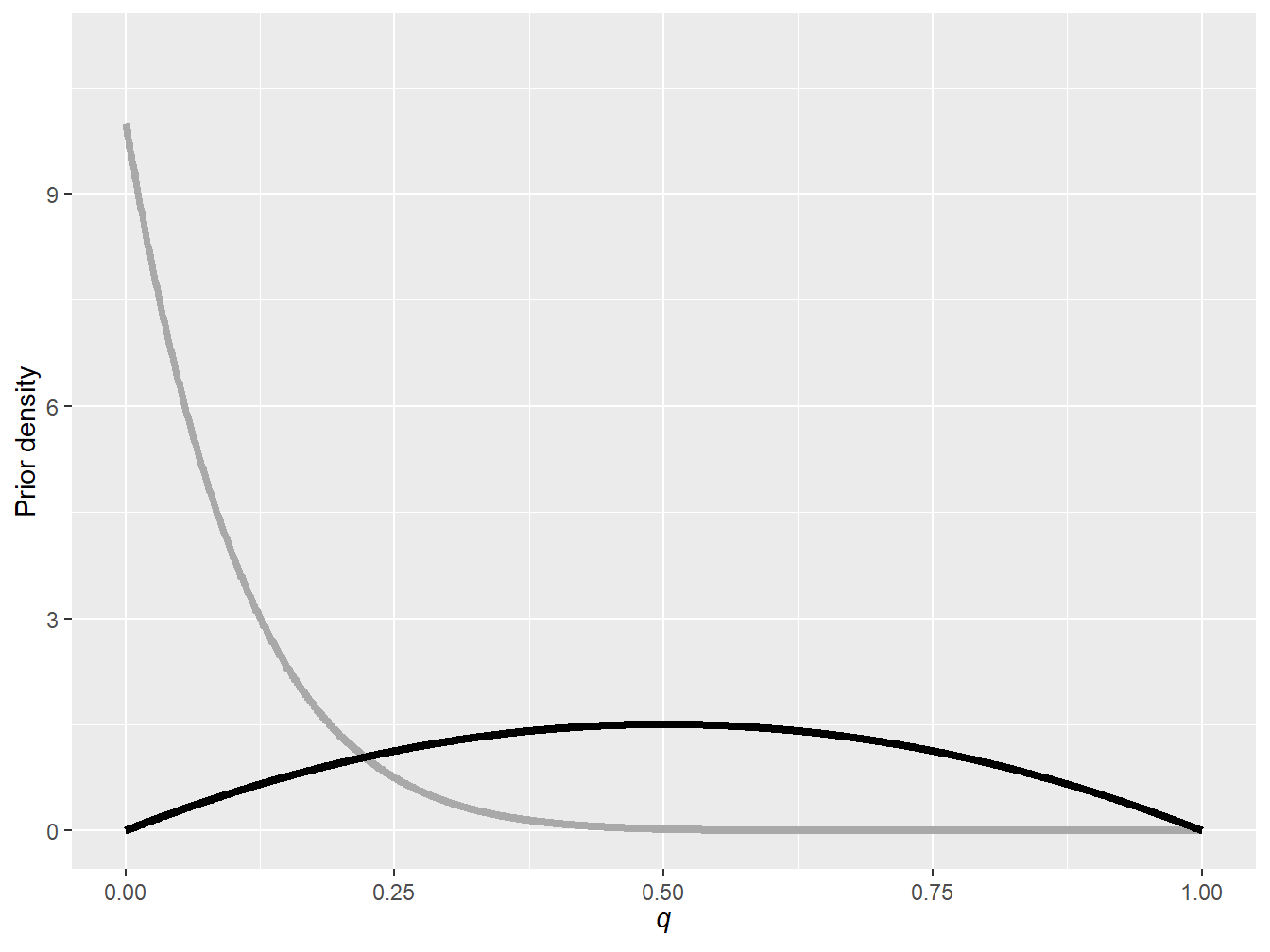
$Beta prior densities: $a=1$ and $b=10$ (gray), and $a=2$ and $b=2$ (black)$

Figure 9.8: Beta prior densities: $a=1$ and $b=10$ (gray), and $a=2$ and $b=2$ (black)

Using again the first 100 lines of the Singapore insurance dataset (see Example 9.1.4 for more details on this dataset), find the two posterior distributions.

Show Example Solution

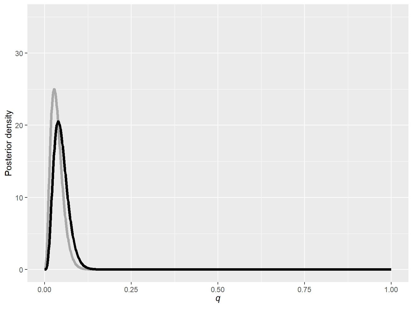
The prior distribution (and its hyperparameters) clearly have an impact on the posterior distribution. As a general rule of thumb for the beta prior, a higher $a$ puts more weight on higher values of $q$ and a higher $b$ puts more weight on lower values of $q$.

9.3.2 The Gamma–Poisson Conjugate Family

We now present a second conjugate family: the gamma–Poisson family. Let $\mathbf{X} = (X_1, X_2, ..., X_n)$ be a sample of iid Poisson random variables such that

\[ p_{X_i|\Lambda=\lambda}(x_i) = \frac{\lambda^{x_i}\, e^{-\lambda}}{x_i!}, \quad x_i \in \mathbb{R}_+ . \]

The likelihood function associated with this sample would therefore be given by

\[ f_{\mathbf{X}|\Lambda=\lambda}(\mathbf{x}) = \prod_{i=1}^n p_{X_i|\Lambda=\lambda}(x_i) = \prod_{i=1}^n \frac{\lambda^{x_i}\, e^{-\lambda}}{x_i!} = \frac{\lambda^x \, e^{-n\lambda}}{\prod_{i=1}^n x_i !} \propto \lambda^x \, e^{-n\lambda}, \]

where $x = \sum_{i=1}^n x_i$. The shape of this likelihood function, as a function of $\lambda$, is reminiscent of a gamma distribution, hinting to the fact that this distribution would be a good contender for a conjugate prior. Indeed, if we let the prior distribution be gamma with shape hyperparameter $\alpha$ and scale hyperparameter $\theta$,

\[ f_{\Lambda}(\lambda) = \frac{1}{\Gamma(\alpha)\theta^{\alpha}} \lambda^{\alpha-1} \, e^{-\frac{\lambda}{\theta}}, \quad \lambda \in \mathbb{R}_+, \]

we can show that the posterior distribution of $\lambda$ is also gamma.

Proposition 9.3.2. Gamma–Poisson Conjugate Family. Consider a sample of $n$ iid Poisson experiments $(X_1,X_2,...,X_n)$, each with rate parameter $\lambda$. Further assume that the random variable associated with the rate, $\Lambda$, has a prior that is gamma distributed with shape hyperparameter $\alpha$ and scale hyperparameter $\theta$. The posterior distribution of $\Lambda$ is therefore given by

\[ f_{\Lambda|\mathbf{X}=\mathbf{x}}(\lambda) = \frac{1}{\Gamma(\alpha+x)\left(\frac{\theta}{n\theta+1} \right)^{\alpha+x}} \lambda^{\alpha+x-1} \, e^{-\frac{\lambda\,(n\theta+1)}{\theta}}, \]

where $x = \sum_{i=1}^n x_i$, which is a gamma distribution with shape parameter $\alpha+x$ and scale parameter $\tfrac{\theta}{n\theta+1}$.

Show A Snippet of Theory

Example 9.3.3. Actuarial Exam Question. You are given:

The number of claims incurred in a month by any insured has a Poisson distribution with mean $\lambda$.
The claim frequencies of different insured are iid.
The prior distribution is gamma with pdf

\[ f_{\Lambda}(\lambda) = \frac{(100\lambda)^6}{120\lambda}e^{-100\lambda}, \quad \lambda \in \mathbb{R}_+. \]

The number of claims every month is distributed as follows:

\[ \begin{matrix} \begin{array}{c|c|c} \hline \text{Month} & \text{Number of Insured} & \text{Number of Claims} \\ \hline \text{1} & 100 & 6 \\\hline \text{2} & 150 & 8 \\\hline \text{3} & 200 & 11 \\\hline \text{4} & 300 & ? \\\hline \end{array} \end{matrix} \]

Calculate the expected number of claims in Month 4.

Show Example Solution

9.3.3 The Normal–Normal Conjugate Family

The last conjugate family is the normal–normal family. Let $\mathbf{X}=(X_1,X_2,...,X_n)$ be a sample of iid normal random variables such that

\[ f_{X_i|M=\mu}(x_i) = \frac{1}{\sqrt{2\pi\sigma^2}}\exp\left( - \frac{1}{2} \frac{(x_i-\mu)^2}{\sigma^2} \right), \quad x_i \in \mathbb{R}. \]

Further, to keep our focus on $\mu$, we will assume throughout our analysis that the variance parameter $\sigma^2$ is known.²¹ The likelihood function associated with this sample would therefore be given by

\[\begin{align} f_{\mathbf{X}|M=\mu}(\mathbf{x}) =&\, \prod_{i=1}^n f_{X_i|M=\mu}(x_i) \\ =&\, \left( \frac{1}{\sqrt{2\pi\sigma^2}} \right)^n \exp\left( - \frac{1}{2} \sum_{i=1}^n \frac{(x_i-\mu)^2}{\sigma^2} \right) \\ \propto&\, \exp\left( - \frac{1}{2} \sum_{i=1}^n \frac{(x_i-\mu)^2}{\sigma^2} \right). \end{align}\]

A very natural prior distribution that matches the likelihood structure is unsurprisingly the normal distribution. Let us assume that the prior distribution for $\mu$ is given by

\[ f_{M}(\mu) = \frac{1}{\sqrt{2\pi \tau^2}} \exp\left( -\frac{1}{2} \frac{(\mu-\theta)^2}{\tau^2} \right), \]

where $\theta$ is the mean parameter and $\tau^2$ is the variance parameter. We can then easily show that the posterior distribution of $\mu$ is also given by a normal distribution.

Proposition 9.3.3. Normal–Normal Conjugate Family. Consider a sample of $n$ iid normals $(X_1,X_2,...,X_n)$, each with mean parameter $\mu$ and variance parameter $\sigma^2$ that is known. Further assume that the random variable associated with the mean, $M$, has a prior that is normally distributed with mean hyperparameter $\theta$ and variance hyperparameter $\tau^2$. The posterior distribution of $M$ is therefore given by

\[ f_{M|\mathbf{X}=\mathbf{x}}(\mu) = \frac{1}{\sqrt{2\pi\left( \frac{\tau^2\sigma^2}{n\tau^2 +\sigma^2} \right)} } \exp\left( - \frac{1}{2} \frac{ \left( \mu - \left( \frac{x}{n} \frac{\tau^2}{n\tau^2 +\sigma^2} + \theta \frac{\sigma^2}{n\tau^2 +\sigma^2} \right) \right)^2 }{ \frac{\tau^2\sigma^2}{n\tau^2 +\sigma^2} } \right), \]

where $x = \sum_{i=1}^n x_i$, which is a normal distribution with mean parameter

\[ \frac{x}{n} \frac{n\tau^2}{n\tau^2 +\sigma^2} + \theta \frac{\sigma^2}{n\tau^2 +\sigma^2} \]

and variance parameter

\[ \frac{\tau^2\sigma^2}{n\tau^2 +\sigma^2}. \]

Show A Snippet of Theory

The prior distribution hyperparameters and posterior distribution parameters can be interpreted in the normal–normal conjugate family:

For the prior, $\theta$ represents the a priori value of the mean parameter, and $\tau^2$ is related to the precisionPrecision is the inverse of variance and is often used to quantify the amount of uncertainty or variability in a prior or posterior distribution. of that prior mean (i.e., the larger the value, the less precise the prior mean is, and vice versa).
For the posterior, the new mean parameter is a weighted average between the prior mean parameter $\theta$ and the sample mean $\tfrac{x}{n}$. The new variance parameter is informed by the prior variability $\tau^2$ and the variability of the data $\sigma^2$.

Example 9.3.4. Impact of Normal Prior on Posterior. Assume the following observed automobile claims for a small portfolio of policies:

\[ 1050, \quad\quad 1250, \quad\quad 1550, \quad\quad 2600, \quad\quad 5350, \quad\quad 10200. \]

Further assume that the logarithm of the claim amount follows a normal distribution with parameters $\mu$ and $\sigma^2 = 1$. Find the posterior distribution of the mean parameter $\mu$ for a normal prior distribution where $\theta = 7$. Consider different values of $\tau^2$; that is, $\tau^2 = 0.1$, $\tau^2 = 1$, and $\tau^2 = 10$. Figure 9.10 shows the pdf of these three prior distributions.

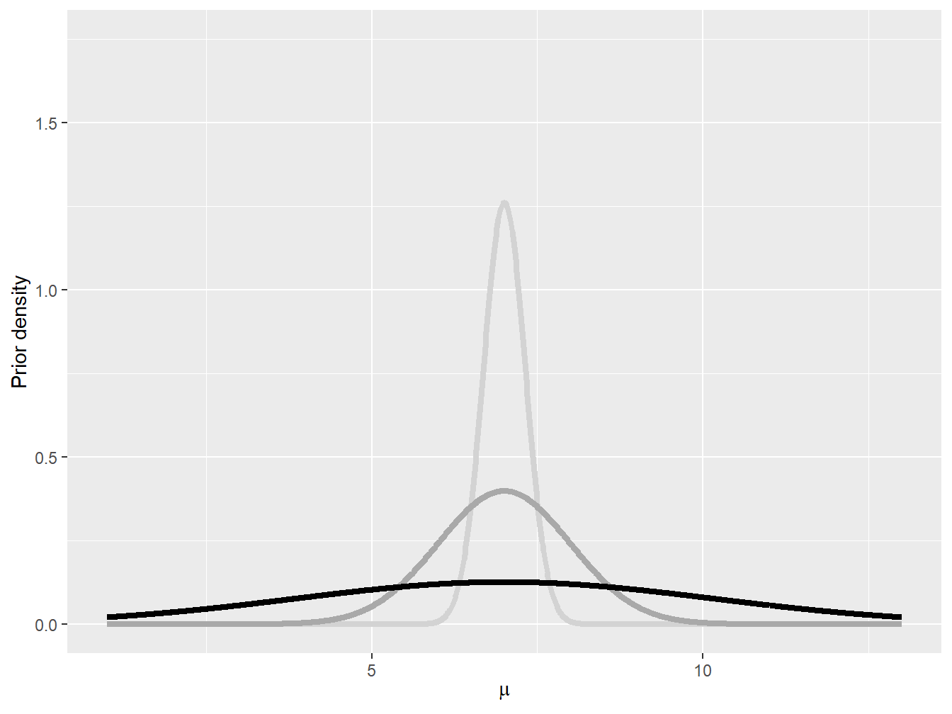
$Normal prior densities: $\tau^2 = 0.1$ (light gray), $\tau^2=1$ (gray), and $\tau^2 = 10$ (black)$

Figure 9.10: Normal prior densities: $\tau^2 = 0.1$ (light gray), $\tau^2=1$ (gray), and $\tau^2 = 10$ (black)

Show Example Solution

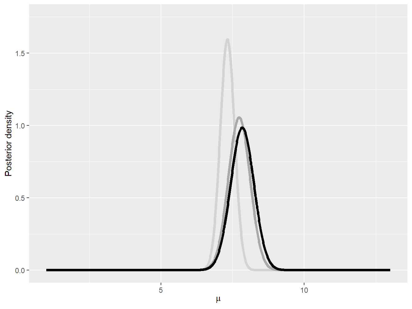
Interestingly, as shown in Example 9.3.4, the prior distribution can have some impact on the final posterior distribution. When the prior assumption about the mean is very precise, having a few data points do not create a huge gap between the prior and the posterior (see the light gray curves in Figures 9.10 and 9.11). When the prior is very imprecise, on the other hand, then the data are allow to speak, and the posterior can be quite different from the prior distribution.

9.3.4 Criticism of Conjugate Family Models

While conjugate family models have some advantages, such as ease of interpretation and computational simplicity, they also have some limitations:

Conjugate families are oftentimes chosen for their mathematical convenience rather than their ability to accurately model the data under study. This can lead to models that are too simplistic and lack the flexibility needed to model real-world phenomena.
Conjugate family models rely on the choice of prior distribution, and different choices of possibly non-conjugate priors can lead to very different posterior distributions.
Conjugate family models are only applicable to a narrow range of problems, which limit their usefulness in practical applications.

It is important to note that while conjugate family models have their limitations, they can still be useful in certain situations, especially when the assumptions of the model are well understood and the data are relatively simple.

9.4 Posterior Simulation

In Section 9.4, you learn how to:

Use the standard computational tools for Bayesian statistics.
Diagnose Markov chain convergence.

9.4.1 Introduction to Markov Chain Monte Carlo Methods

Sometimes, using conjugate family models is ill-suited for the problem at hand, and more complicated priors need to be selected. Under other circumstances, complex models involve many parameters making the posterior distribution intractable. In these cases, the posterior distribution of the parameters will not have a closed-form solution, generally speaking, and will need to be estimated via numerical methods.

A common way to generate draws of the parameter posterior distribution is to create Markov chains for which their stationary distributions—the probability distribution that remains unchanged when the Markov chain has reached a state where the transition probabilities no longer evolve over time—correspond to the posterior of interest. These Markov chain-based methods are known as Markov chain Monte Carlo (MCMC) methods in the literature. This section provides a brief overview of these methods and of their uses. We do not intend to give much of the theory behind these methods, which would require a deep understanding of Markov chains and their theory.²² Instead, we focus on their applications in insurance and loss modeling. Specifically, in the next two subsections, we introduce the two most common MCMC methods; that is, the Gibbs samplerThe Gibbs sampler is an iterative algorithm in statistics used for simulating samples from complex probability distributions. It’s particularly useful in Bayesian analysis for drawing samples from multivariate distributions by updating one variable at a time while keeping others fixed. of Gelfand and Smith (1990) and the Metropolis–Hastings algorithmThe Metropolis–Hastings algorithm is a method to generate samples from complex distributions by proposing new samples and deciding whether to accept them, making it valuable for Bayesian analysis and complex modeling. of Hastings (1970) and Metropolis et al. (1953).

9.4.2 The Gibbs Sampler

As mentioned above, sometimes, we cannot use conjugate families. In other cases where the parameter space is large, it can be very hard to find the marginal likelihood $f_{\mathbf{X}}(\mathbf{x})$ (also known as the normalizing constant); that is, assuming that the model parameters are given by $\pmb{\theta} = [\, \theta_1 \quad ... \theta_2 \quad ... \quad \theta_k \,]$ and contains $k$ parameters, the marginal likelihood given by

\[ f_{\mathbf{X}}(\mathbf{x}) = \int \int ... \int f_{\mathbf{X}|\pmb{\Theta} = \pmb{\theta}} (\mathbf{x}) f_{\pmb{\Theta}}(\pmb{\theta}) \, d\theta_1 \,d\theta_2 \,... \,d\theta_k \]

is hard to compute even when using typical quadrature-based rules, especially if $k$ is large.

Fortunately, under very mild regularity conditions, samples of the joint estimates of parameters can be obtained by sequentially sampling each parameter individually and by keeping all the other parameters constant. To do so, the distribution of any given parameter conditional on all the other parameters (and the data) needs to be known. These distributions are known as full conditional distributions; that is,

\[ f_{\Theta_i \,|\, \mathbf{X} = \mathbf{x}, \, \pmb{\Theta}_{\backslash i} = \pmb{\theta}_{\backslash i}} (\theta_i), \]

for parameter $\theta_i$, where $\pmb{\theta}_{\backslash i}$ represents all parameters except for the $i^{\text{th}}$ one, and $\pmb{\Theta}_{\backslash i}$ is the random variable associated with this set of parameters.

The full conditional distribution is an important building block in Gibbs sampling. Indeed, if one can obtain each parameter’s distribution conditional on having the value of all the other parameters in closed form, then it is possible to generate samples for each parameter. Specifically, starting from an arbitrary set of starting values $\pmb{\theta}^{(0)}_{\vphantom{2}} = [ \, {\theta}_1^{(0)} \quad {\theta}_2^{(0)} \quad ... \quad {\theta}_k^{(0)} \, ]$, samples for each parameter can be generated by performing the following steps for $m = 1, 2, ..., M$:

Draw $\theta^{(m)}_1$ from $f_{\Theta_1^{\vphantom{(m)}} \, |\, \mathbf{X} = \mathbf{x}, \, \Theta_2^{\vphantom{(m)}} = \, \theta_2^{(m-1)}, \,..., \, \Theta_k^{\vphantom{(m)}} = \, \theta_k^{(m-1)}} (\theta_1)$.
Draw $\theta^{(m)}_2$ from $f_{\Theta_2^{\vphantom{(m)}} \, |\, \mathbf{X} = \mathbf{x}, \, \Theta_1^{\vphantom{(m)}} = \, \theta_1^{(m)}, \, \Theta_3^{\vphantom{(m)}} = \,\theta_3^{(m-1)}, \,..., \, \Theta_k^{\vphantom{(m)}} = \,\theta_k^{(m-1)}} (\theta_2)$.
Draw $\theta^{(m)}_3$ from $f_{\Theta_3^{\vphantom{(m)}} \, |\, \mathbf{X} = \mathbf{x}, \, \Theta_1^{\vphantom{(m)}} =\, \theta_1^{(m)}, \, \Theta_2^{\vphantom{(m)}} =\, \theta_2^{(m)}, \, \Theta_4^{\vphantom{(m)}} = \,\theta_4^{(m-1)}, \,..., \, \Theta_k^{\vphantom{(m)}} =\, \theta_k^{(m-1)}} (\theta_3)$.

$\vdots$

$k$. Draw $\theta^{(m)}_k$ from $f_{\Theta_k^{\vphantom{(m)}} \, |\, \mathbf{X} = \mathbf{x}, \, \Theta_1^{\vphantom{(m)}} =\, \theta_1^{(m)}, \,..., \, \Theta_{k-1}^{\vphantom{(m)}} = \,\theta_{k-1}^{(m)}} (\theta_k)$.

The sample, especially at first, will depend on the initial values, $\pmb{\theta}^{(0)}_{\vphantom{2}}$, and it might take some time until the sampler can get to the stationary distribution. For this reason, in practice, experimenters discard the first $M^*$ iterations to make sure their analysis is not impacted by the choice of initial parameter; this initial period of discarded sample is known as the burn-in period.

The rest of the sample—the remaining $M-M^*$ iterations—is kept to estimate the posterior distribution and any quantities of interest.

9.4.2.1 Application to Bayesian Linear Regression

In statistics and in its most simple form, a linear regression is an approach for modeling the relationship between a scalar response and an explanatory variable. The former quantity is denoted by $x_i$ for $i \in \{1, ..., n\}$, and the latter quantity is denoted by $z_{i}$ for $i \in \{1,...,n\}$ in this chapter. Mathematically, we can write this relationship as

\[ x_i = \alpha + \beta z_{i} + \varepsilon_i, \]

where $\varepsilon_i$ is a disturbance term that captures the potential for errors in the linear relationship. This error term is typically assumed to be normally distributed with mean zero and variance $\sigma^2$.

In general, the coefficients $\alpha$ and $\beta$ are unknown and need to be estimated. The experimenter can rely on Bayesian statistics to find out the posterior distribution of the parameters $\alpha$ and $\beta$ along with that of $\sigma^2$. For the rest of the subsection, we investigate a specific application of Gibbs sampling to the context of linear regression.

We begin by computing the likelihood function conditional on the parameter values:

\[\begin{align*} f_{\mathbf{X}\,|\,A=\alpha,\, B=\beta,\,\Sigma^2=\sigma^2}(\mathbf{x})=&\, \prod_{i=1}^n \frac{1}{\sqrt{2\pi\sigma^2}} \exp\left( - \frac{\left( x_i - \alpha -\beta z_{i} \right)^{2}}{2 \sigma^2} \right) \\ =&\, \left( 2 \pi \sigma^2 \right)^{-\tfrac{n}{2}} \exp\left(- \frac{\sum_{i=1}^n \left( x_i - \alpha - \beta z_{i} \right)^{2}}{2 \sigma^2} \right), \end{align*}\]

which is the first building block to construct our posterior distribution.

Then, we need a prior distribution, which could be informative, weakly informative, or noninformative. In this application, we select a prior that allows us to obtain each parameter’s full conditional distribution in closed form. Specifically, we use a normal distribution for $\alpha$ and $\beta$, and an inverse gamma distribution for $\sigma^2$ with shape parameter $\tfrac{n_{\sigma}}{2}$ and scale parameter $\tfrac{\theta_{\sigma}}{2}$, where

\[\begin{align*} f_{A}(\alpha) =&\, \frac{1}{\sqrt{2\pi \tau_{\alpha}^2\vphantom{2\pi \tau_{\beta}^2} }} \exp\left( - \frac{1}{2} \frac{(\alpha-\theta_{\alpha})^2}{\tau_{\alpha}^2 } \right), \\ f_{B}(\beta) =&\, \frac{1}{\sqrt{2\pi \tau_{\beta}^2 }} \exp\left( - \frac{1}{2} \frac{(\beta-\theta_{\beta})^2}{\tau_{\beta}^2 } \right), \\ f_{\Sigma^2}(\sigma^2) =&\, \frac{(\theta_{\sigma}/2)^{n_{\sigma}/2}}{\Gamma(n_{\sigma}/2)} \left( \frac{1}{\sigma^2} \right)^{n_{\sigma}/2+1} \exp\left( - \frac{\theta_{\sigma}/2}{\sigma^2} \right). \end{align*}\]

Proposition 9.4.1. Full Conditional Distributions of Bayesian Linear Regression Parameters. Consider a sample of $n$ observations $\mathbf{x} = (x_1,...,x_n)$ for which

\[ x_i = \alpha + \beta z_{i} + \varepsilon_i, \]

where $\varepsilon_i$ is normally distributed with mean zero and variance $\sigma^2$. The full conditional distributions of parameters $\alpha$, $\beta$, and $\sigma^2$ are given by the following expressions:

\[\begin{align*} A\sim&\, \text{Normal}\left( \frac{1}{n} \left(\sum_{i=1}^n x_i - \beta z_i \right) \frac{n \tau_{\alpha}^2}{n\tau_{\alpha}^2 + \sigma^2} + \theta_{\alpha} \frac{\sigma^2}{n\tau_{\alpha}^2+\sigma^2}, \frac{\tau_{\alpha}^2\sigma^2}{n\tau_{\alpha}^2+\sigma^2} \right), \\ B\sim&\, \text{Normal}\left( \frac{1}{n}\left( \sum_{i=1}^n z_i\left( x_i - \alpha \right) \right) \frac{n \tau_{\beta}^2}{\tau_{\beta}^2\sum_{i=1}^n z_i^2 + \sigma^2} + \theta_{\beta} \frac{\sigma^2}{\tau_{\beta}^2\sum_{i=1}^n z_i^2 +\sigma^2}, \frac{\tau_{\beta}^2\sigma^2}{\tau_{\beta}^2 \sum_{i=1}^n z_i^2 +\sigma^2} \right)\!, \\ \Sigma^2\sim &\, \text{Inverse Gamma}\left( \frac{n_{\sigma}+n}{2}, \frac{\theta_{\sigma} + \sum_{i=1}^n \left( y_i - \alpha - \beta z_{i} \right)^{2}}{2} \right), \end{align*}\]

respectively, assuming the prior distributions mentioned above.

Show A Snippet of Theory

Proof. From Section 9.2, we know that

\[ f_{A,B,\Sigma^2|\mathbf{X}=\mathbf{x}}(\alpha,\beta,\sigma^2) \propto f_{\mathbf{X}|A=\alpha,\, B=\beta,\,\Sigma^2=\sigma^2}(\mathbf{x})\, f_{A}(\alpha)\, f_{B}(\beta) \, f_{\Sigma^2}(\sigma^2), \]

which is useful to derive the full conditional distributions of $\alpha$, $\beta$, and $\sigma^2$.

Let us begin with $\alpha$:

\[\begin{align*} &\, f_{A|\mathbf{X}=\mathbf{x},\,B=\beta,\,\Sigma^2=\sigma^2}(\alpha) \\ \propto&\, \exp\left(- \frac{1}{2}\frac{\sum_{i=1}^n \left( x_i - \alpha - \beta z_{i} \right)^{2}}{\sigma^2} \right) \exp\left( - \frac{1}{2} \frac{(\alpha-\theta_{\alpha})^2}{\tau_{\alpha}^2 } \right) \\ \propto &\,\exp\left(-\frac{1}{2} \left( \frac{n \alpha^2 - 2 \alpha \sum_{i=1}^n (x_i - \beta z_i)}{\sigma^2} + \frac{\alpha^2 -2\alpha \theta_{\alpha} }{\tau_{\alpha}^2} \right) \right) \\ \propto &\,\exp\left( -\frac{1}{2} \left( \frac{\alpha^2 - 2 \alpha \left( \frac{1}{n}\left( \sum_{i=1}^n x_i - \beta z_i \right) \frac{n \tau_{\alpha}^2}{n\tau_{\alpha}^2 + \sigma^2} + \theta_{\alpha} \frac{\sigma^2}{n\tau_{\alpha}^2+\sigma^2}\right)}{\frac{\tau_{\alpha}^2\sigma^2}{n\tau_{\alpha}^2+\sigma^2}} \right) \right) \\ \propto &\,\frac{1}{\sqrt{2\pi \left(\frac{\tau_{\alpha}^2\sigma^2}{n\tau_{\alpha}^2+\sigma^2}\right)}} \exp\left( -\frac{1}{2} \left( \frac{\left(\alpha - \left( \frac{1}{n}\left( \sum_{i=1}^n x_i - \beta z_i \right) \frac{n \tau_{\alpha}^2}{n\tau_{\alpha}^2 + \sigma^2} + \theta_{\alpha} \frac{\sigma^2}{n\tau_{\alpha}^2+\sigma^2}\right)\right)^2}{\frac{\tau_{\alpha}^2\sigma^2}{n\tau_{\alpha}^2+\sigma^2}} \right) \right) \end{align*}\]

which is a normal distribution with mean parameter

\[ \frac{1}{n} \left(\sum_{i=1}^n x_i - \beta z_i \right) \frac{n \tau_{\alpha}^2}{n\tau_{\alpha}^2 + \sigma^2} + \theta_{\alpha} \frac{\sigma^2}{n\tau_{\alpha}^2+\sigma^2} \]

and variance parameter

\[ \frac{\tau_{\alpha}^2\sigma^2}{n\tau_{\alpha}^2+\sigma^2}. \]

The derivation to obtain the full conditional distribution of $\beta$ is similar to that of $\alpha$:

\[\begin{align*} &\, f_{B|\mathbf{X}=\mathbf{x},\,A=\alpha,\,\Sigma^2=\sigma^2}(\beta) \\ \propto&\, \exp\left(- \frac{1}{2}\frac{\sum_{i=1}^n \left( x_i - \alpha - \beta z_{i} \right)^{2}}{\sigma^2} \right) \exp\left( - \frac{1}{2} \frac{(\beta-\theta_{\beta})^2}{\tau_{\beta}^2 } \right) \\ \propto &\,\exp\left(-\frac{1}{2} \left( \frac{\beta^2 \sum_{i=1}^n z_i^2 - 2 \beta \sum_{i=1}^n z_i (x_i - \alpha)}{\sigma^2} + \frac{\beta^2 -2\beta \theta_{\beta} }{\tau_{\beta}^2} \right) \right) \\ \propto &\,\exp\left( -\frac{1}{2} \left( \frac{\beta^2 - 2 \beta \left( \frac{1}{n}\left( \sum_{i=1}^n z_i \left( x_i - \alpha \right) \right) \frac{n \tau_{\beta}^2}{\tau_{\beta}^2 \sum_{i=1}^n z_i^2 + \sigma^2} + \theta_{\beta} \frac{\sigma^2}{\tau_{\beta}^2\sum_{i=1}^n z_i^2+\sigma^2}\right)}{\frac{\sigma_{\beta}^2\sigma^2}{\tau_{\beta}^2 \sum_{i=1}^n z_i^2+\sigma^2}} \right) \right) \\ \propto &\,\frac{1}{\sqrt{2\pi \left(\frac{\tau_{\beta}^2\sigma^2}{\tau_{\beta}^2 \sum_{i=1}^n z_i^2 +\sigma^2}\right)}} \\ &\, \times \exp\left( -\frac{1}{2} \left( \frac{\left(\beta - \left( \frac{1}{n}\left( \sum_{i=1}^n z_i\left( x_i - \alpha \right) \right) \frac{n \tau_{\beta}^2}{\tau_{\beta}^2\sum_{i=1}^n z_i^2 + \sigma^2} + \theta_{\beta} \frac{\sigma^2}{\tau_{\beta}^2\sum_{i=1}^n z_i^2 +\sigma^2}\right)\right)^2}{\frac{\tau_{\alpha}^2\sigma^2}{\tau_{\beta}^2 \sum_{i=1}^n z_i^2+\sigma^2}} \right) \right) \end{align*}\]

which is a normal distribution with mean parameter

\[ \frac{1}{n}\left( \sum_{i=1}^n z_i\left( x_i - \alpha \right) \right) \frac{n \tau_{\beta}^2}{\tau_{\beta}^2\sum_{i=1}^n z_i^2 + \sigma^2} + \theta_{\beta} \frac{\sigma^2}{\tau_{\beta}^2\sum_{i=1}^n z_i^2 +\sigma^2} \]

and variance parameter

\[ \frac{\tau_{\beta}^2\sigma^2}{\tau_{\beta}^2 \sum_{i=1}^n z_i^2 +\sigma^2}. \]

Finally, we apply the same logic to the variance parameter, $\sigma^2$:

\[\begin{align*} &\,f_{\Sigma^2|\mathbf{X}=\mathbf{x},\,A=\alpha,\,B=\beta}(\sigma^2) \\ \propto&\, \left( 2 \pi \sigma^2 \right)^{-n/2} \exp\left(- \frac{1}{2}\frac{\sum_{i=1}^n \left( x_i - \alpha - \beta z_{i} \right)^{2}}{\sigma^2} \right) \left( \frac{1}{\sigma^2} \right)^{n_{\sigma}/2+1} \exp\left( - \frac{\theta_{\sigma}/2}{\sigma^2} \right) \\ \propto&\, \exp\left(- \frac{1}{2}\frac{\theta_{\sigma} + \sum_{i=1}^n \left( x_i - \alpha - \beta z_{i} \right)^{2}}{\sigma^2} \right) \left( \frac{1}{\sigma^2} \right)^{(n_{\sigma}+n)/2+1} \\ \propto &\, \frac{\left(\frac{\theta_{\sigma} + \sum_{i=1}^n \left( x_i - \alpha - \beta z_{i} \right)^{2}}{2}\right)^{(n_{\sigma}+n)/2}}{\Gamma((n_{\sigma}+n)/2)} \left( \frac{1}{\sigma^2} \right)^{(n_{\sigma}+n)/2+1} \exp\left( - \frac{\frac{\theta_{\sigma} + \sum_{i=1}^n \left( x_i - \alpha - \beta z_{i} \right)^{2}}{2}}{\sigma^2} \right), \end{align*}\]

which is an inverse gamma distribution with shape parameter $\tfrac{n_{\sigma}+n}{2}$ and scale parameter

\[ \frac{\theta_{\sigma} + \sum_{i=1}^n \left( x_i - \alpha - \beta z_{i} \right)^{2}}{2}. \]

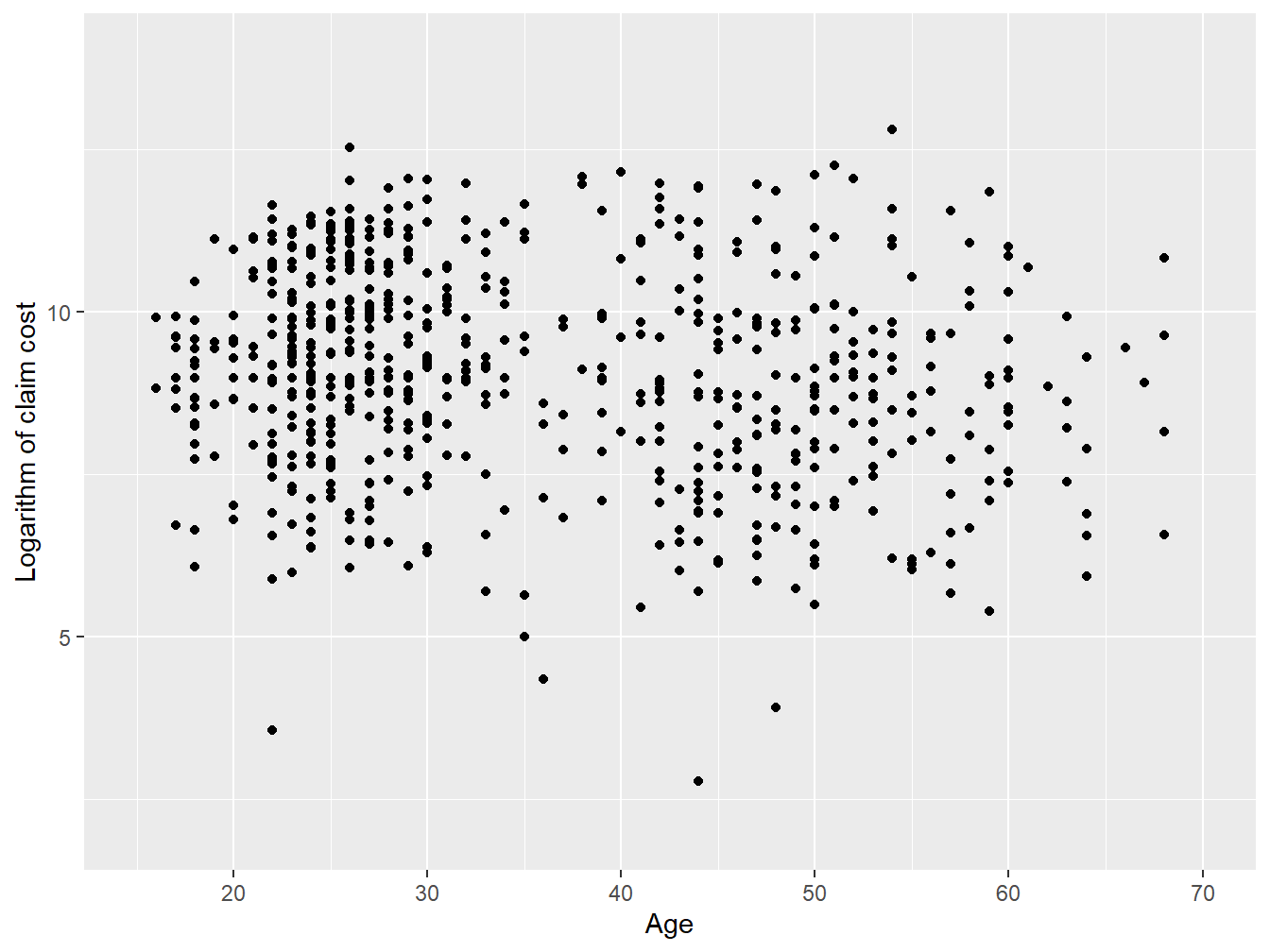
We now apply the Gibbs sampler on real data. The example will use motorcycle insurance data from Wasa, a Swedish insurance company, taken from dataOhlsson of the R package insuranceData; see Wolny-Dominiak and Trzesiok (2014) for more details.

library("insuranceData")
data(dataOhlsson)

This dataset contains information about the number of motorcycle accidents, their claim cost, and some risk factors (e.g., the age of the driver, the age of the vehicle, the geographic zone).

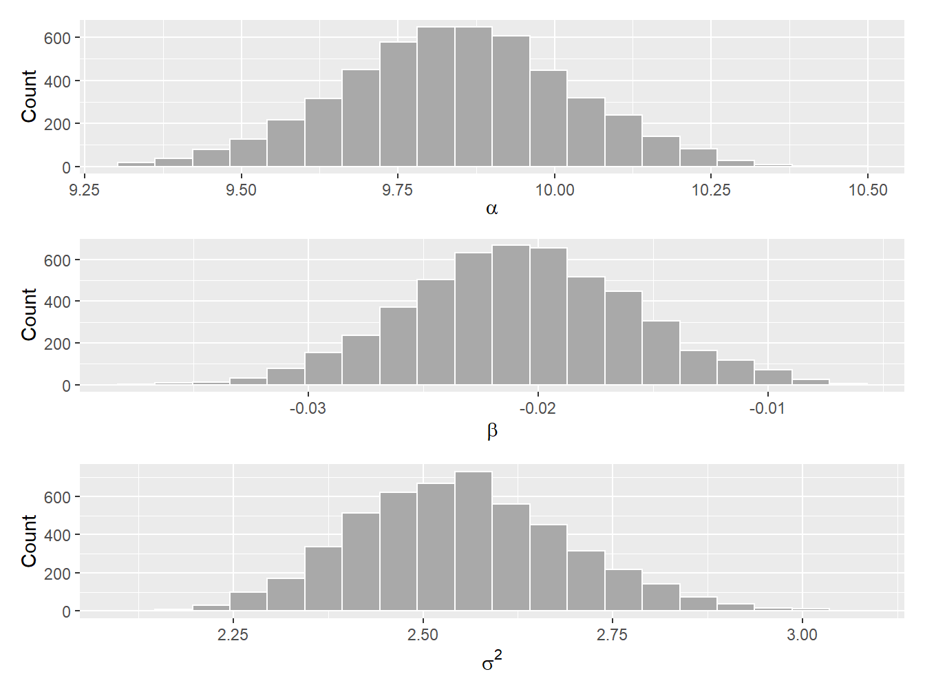
Example 9.4.1. Bayesian Linear Regression. You wish to understand the relationship between the age of the driver and the (logarithm of the) claim cost. Let $x_i$ be the logarithm of the $i^{\text{th}}$ claim cost and $z_i$ be the age associated with the $i^{\text{th}}$ claim. Further assume the following linear relationship between the two quantities:

\[ x_i = \alpha + \beta z_{i} + \varepsilon_i, \]

where $\varepsilon_i$ is normally distributed with mean zero and variance $\sigma^2$. Find the posterior density of the three parameters $\alpha$, $\beta$, and $\sigma^2$ using the Gibbs sampler.

Show Example Solution

Solution. Let us begin by visualizing the data. Figure 9.12 reports the logarithm of the claim cost as a function of the driver’s age. At first sight, it seems that the relationship between the claim cost and age is negative, so we should expect a negative $\beta$, generally speaking.

Figure 9.12: Logarithm of the claim cost as a function of the driver’s age

Let us now turn to Bayesian computation via Gibbs sampling to find the posterior distribution of the three parameters of interest. We will use 10,000 iterations and discard the first 5,000 iterations (i.e., burn-in period). For our prior distributions, we use weakly informative priors by setting $\theta_{\alpha} = \tfrac{1}{n} \sum_{i=1}^n x_i = \overline{x}$, $\theta_{\beta} = 0$, $\tau_{\alpha}^2=\tau_{\beta}^2 = 10$, $n_{\sigma} = 1$, and $\theta_{\sigma} = 0.1$. The initial values of the parameters are set to: $\alpha^{(0)} = \overline{x}$, $\beta^{(0)} = 0$, and $\sigma^{2\,(0)} = \tfrac{1}{n} \sum_{i=1}^n (x_i - \overline{x})^2$.

set.seed(1)
library("nimble")
dataOhlsson <- dataOhlsson[dataOhlsson$skadkost > 0, ]
dataOhlsson$logskadkost <- log(dataOhlsson$skadkost)

x <- dataOhlsson$logskadkost
z <- dataOhlsson$agarald

n <- length(x)
M <- 10000
Mstar <- 5000
thetaa <- mean(x)
tau2a <- 10
thetab <- 0
tau2b <- 10
nsigma <- 1
thetasigma <- 0.1

alphas <- rep(NA, M + 1)
betas <- rep(NA, M + 1)
sigma2s <- rep(NA, M + 1)

alphas[1] <- mean(x)
betas[1] <- 0
sigma2s[1] <- var(x)

for (m in 2:(M + 1)) {
    # Generate alpha
    den_alpha <- n * tau2a + sigma2s[m - 1]
    mean_alpha <- (1/n) * (sum(x - betas[m - 1] * z)) * (n * tau2a)/den_alpha + thetaa *
        sigma2s[m - 1]/den_alpha
    var_alpha <- tau2a * sigma2s[m - 1]/den_alpha

    alphas[m] <- rnorm(1, mean = mean_alpha, sd = sqrt(var_alpha))

    # Generate beta
    den_beta <- tau2b * sum(z^2) + sigma2s[m - 1]
    mean_beta <- (1/n) * (sum(z * (x - alphas[m]))) * (n * tau2b)/den_beta + thetab *
        sigma2s[m - 1]/den_beta
    var_beta <- tau2b * sigma2s[m - 1]/den_beta

    betas[m] <- rnorm(1, mean = mean_beta, sd = sqrt(var_beta))

    # Generate sigma^2
    shape_sigma <- (nsigma + n)/2
    scale_sigma <- (thetasigma + sum((x - alphas[m] - betas[m] * z)^2))/2

    sigma2s[m] <- rinvgamma(1, shape = shape_sigma, scale = scale_sigma)
}

Once we have the posterior parameter samples, we can get multiple quantities of interest. For instance, the posterior mean of parameters $\alpha$, $\beta$, and $\sigma^2$ are $9.843$, $-0.0208$, and $2.551$, respectively. These posterior means are obtained by simply taking the sample means of the respective posterior draws; that is, these are Monte Carlo estimates of the posterior means.

The posterior mean for coefficient alpha is 9.84259435

The posterior mean for coefficient beta is -0.0207847772

The posterior mean for the variance parameter is 2.55090494

We can also get histograms of the posterior distribution for $\alpha$, $\beta$, and $\sigma^2$; Figure 9.13 reports histograms for the three parameters. The uncertainty around each parameter is very small.

$Histogram of the posterior distribution for parameters $\alpha$ (top panel), $\beta$ (middle panel), and $\sigma^2$ (bottom panel)$

Figure 9.13: Histogram of the posterior distribution for parameters $\alpha$ (top panel), $\beta$ (middle panel), and $\sigma^2$ (bottom panel)

The top panel of Figure 9.14 reports a plot of the post-burn-in values of $\alpha$ as a function of the iteration number; this type of plot is known as a trace plot in the literature. These samples are not impacted by the initial parameter value that was selected. Indeed, after about 20–30 iterations, the posterior parameter values obtained by the Gibbs sampler are very close to their posterior means. For instance, the bottom panel of Figure 9.14 shows a plot of the first 50 values of $\alpha$ as a function of the iteration number.

$Trace plot of $\alpha$ for the post-burn-in iterations (top panel) and for the first 50 iterations (bottom panel)$

Figure 9.14: Trace plot of $\alpha$ for the post-burn-in iterations (top panel) and for the first 50 iterations (bottom panel)

9.4.3 The Metropolis–Hastings Algorithm

Gibbs sampling works well when the full conditional distribution for each parameter in the model can be found and is of a common form. This, unfortunately, is not always possible, meaning that we need to rely on other computational tools to find the posterior distribution of the parameters. One very popular method that copes with the shortcomings of Gibbs’ method is the Metropolis–Hastings sampler.

Let us assume that the current value of the first model parameter is $\theta_1^{(0)}$. From this current value, we now wish to find a new value for this parameter. To do so, we propose a new value for this parameter, $\theta^*_1$, from a candidate (or proposal) density $q\left( \theta_1^* \,\middle|\, \theta_1^{(0)} \right)$. Since this proposal has nothing to do with the posterior distribution of the parameter, we should not keep all candidates in our final sample—we only accept those samples that are representative of the posterior distribution of interest. To determine whether we accept or reject the candidate, we compute a so-called acceptance ratio $\alpha\left( \theta_1^{(0)}, \theta_1^* \right)$ using

\[ \alpha\left(\theta_1^{(0)},\theta_1^*\right) = \frac{h\left(\theta_1^*\vphantom{\theta_1^{(1)}}\right) q\left( \theta_1^{(0)} \,\middle|\,\theta_1^* \right)}{h\left(\theta_1^{(1)}\right) q\left( \theta_1^* \,\middle|\, \theta_1^{(0)} \right)} \]

where

\[ h(\theta_1) = f_{\mathbf{X}\,|\,\Theta_1 = \,\theta_1, \, \pmb{\Theta}_{\backslash1}=\,\pmb{\theta}_{\backslash1}}(\mathbf{x}) \, f_{\Theta_1,\pmb{\Theta}_{\backslash1}}\left(\theta_1,\pmb{\theta}_{\backslash1}\right) \]

and $\pmb{\theta}_{\backslash 1}$ represents all parameters except for the first one. Then, we accept the proposed value $\theta_1^*$ with probability $\alpha\left( \theta_1^{(0)}, \theta_1^* \right)$ and reject it with probability $1-\alpha\left( \theta_1^{(0)}, \theta_1^* \right)$. Specifically,

\[ \theta_1^{(1)} = \left\{ \begin{array}{ll} \theta_1^* & \text{with probability }\,\alpha\left(\theta_1^{(0)},\theta_1^*\right) \\ \theta_1^{(0)} &\text{with probability }\,1-\alpha\left(\theta_1^{(0)},\theta_1^*\right) \end{array} \right. \]

We can repeat the same process for all other parameters to obtain $\theta_2^{(1)}$ to $\theta_k^{(1)}$, while replacing the parameters $\pmb{\theta}_{\backslash i}$ by their most current values in the chain. Once we have updated all values, we can repeat this process for all $m$ in $\{2,3,...,M\}$, similar to the iterative process used in the Gibbs sampler.²³

Special Case: Symmetric Proposal Distribution. If a proposal distribution is symmetric, then

\[ q\left( \theta_i^{(m)} \,\middle|\,\theta_i^* \right) = q\left( \theta_i^* \,\middle|\,\theta_i^{(m)} \right), \]

and those terms cancel out, leaving

\[ \alpha\left(\theta_i^{(m)},\theta_1^*\right) = \frac{h\left(\theta_i^*\vphantom{\theta_1^{(1)}}\right)}{h\left(\theta_i^{(m)}\right) }. \]

This special case is called the Metropolis algorithm.

The Metropolis–Hastings sampler requires a lot of fine-tuning, generally speaking, because the experimenter needs to select a proposal distribution for each parameter. A common approach is to assume a normal proposal distribution centered at the previous value; that is,

\[ \Theta_i^* \sim \text{Normal}\left( \theta_i^{(m-1)} , \delta_i^2 \right), \]

at step $m$, where $\delta_i^2$ is the variance of the $i^{\text{th}}$ parameter’s proposal distribution.

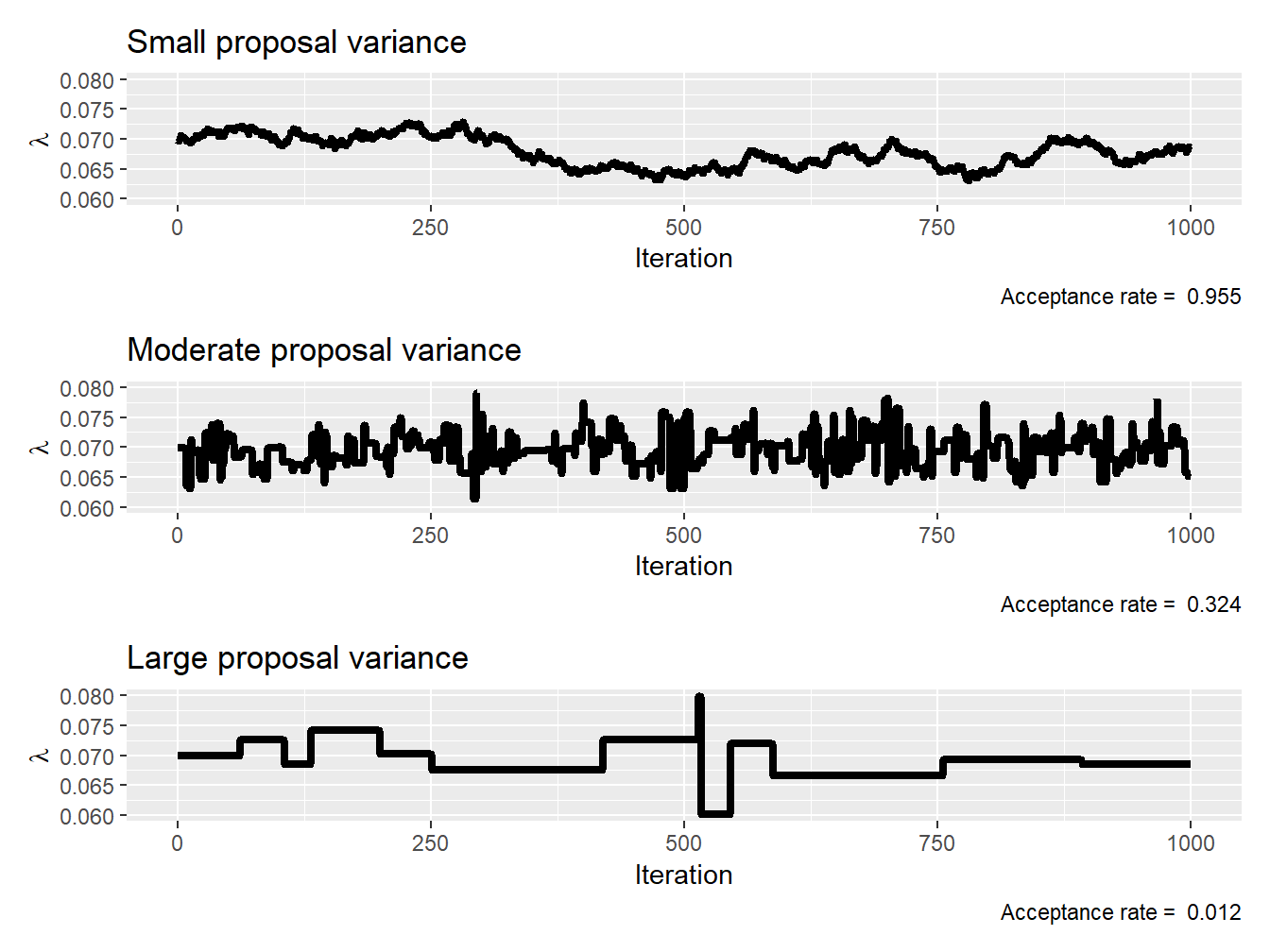
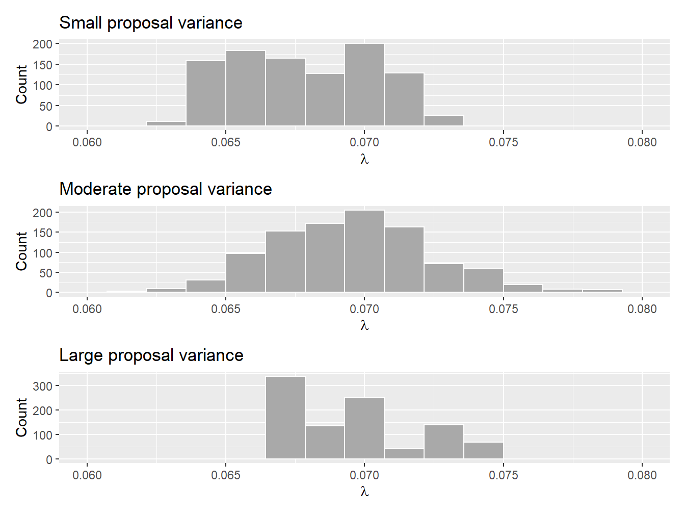
Example 9.4.2. Impact of Proposal Density on the Acceptance Rate. Assume that each policyholder’s claim count (frequency) is distributed as a Poisson random variable such that

\[ p_{N_i\,|\,\Lambda=\lambda}(n_i) = \frac{\lambda^{n_i}e^{-\lambda}}{n_i!}, \]

where $n_i$ is the number of claims associated with the $i^{\text{th}}$ policyholder. Further assume a noninformative, flat prior over $[0,\infty]$; that is,

\[ f_{\Lambda}(\lambda) \propto 1, \quad \lambda \in [0,\infty]. \]

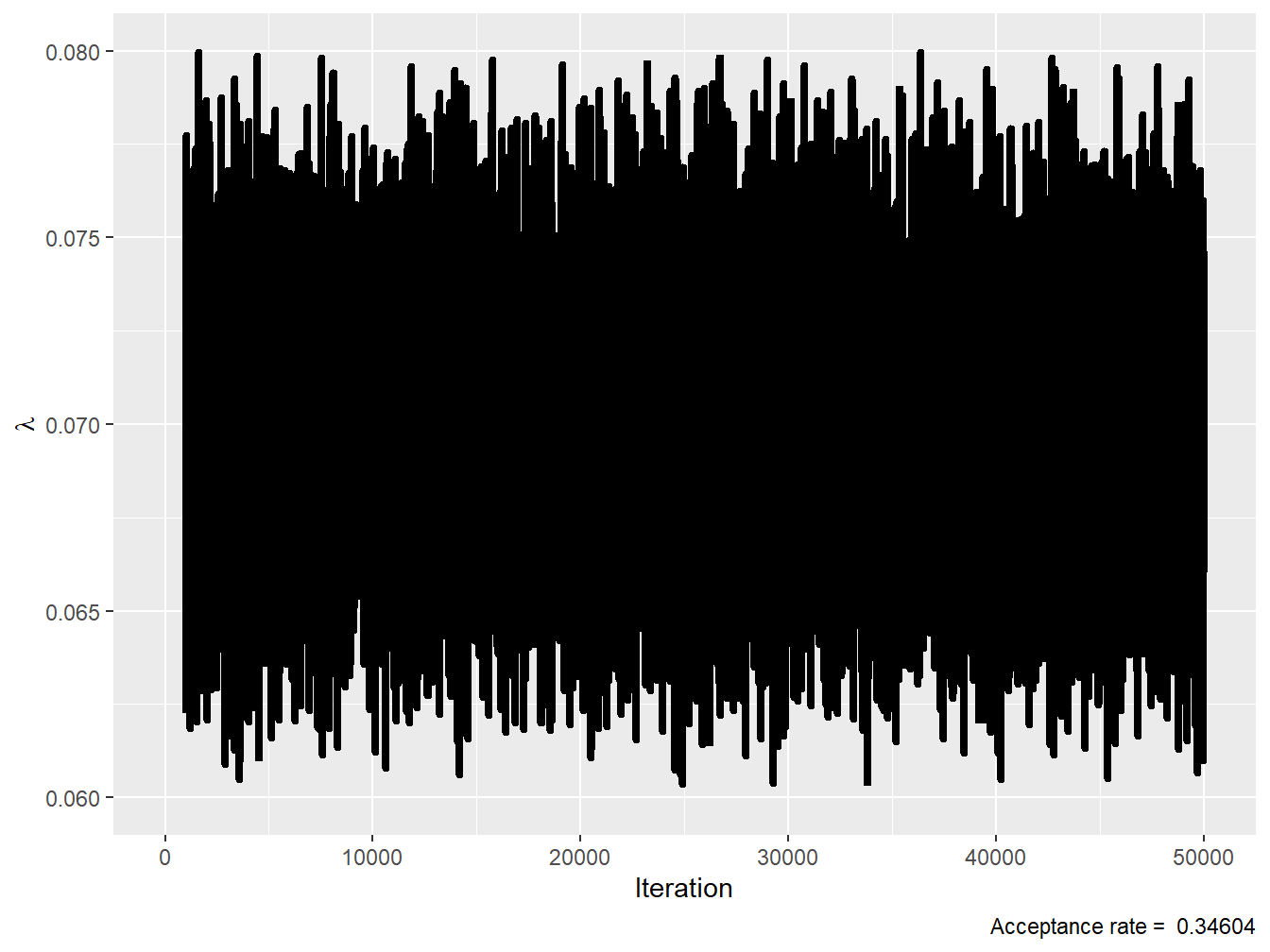
Find the posterior distribution of the parameter using 1,000 iterations of the Metropolis–Hastings sampler assuming the claim count data of the Singapore Insurance Data (see Example 9.1.4 for more details). Use a normal proposal with small ($1\times 10^{-7}$), moderate ($1\times 10^{-4}$), and large ($1 \times 10^{-1}$) values as the proposal variance $\delta$ in your tests and comment on the differences.

Show Example Solution

Solution. Starting from the the likelihood function and the prior distribution, we have that

\[ h(\lambda) \propto \prod_{i=1}^N \frac{\lambda^{n_i}e^{-\lambda}}{n_i!}. \]

M <- 1000

# First variance: 1 x 10^-7
set.seed(1)
delta21 <- 0.0000001

lambdas1 <- rep(NA, M + 1)
lambdas1[1] <- mean(sgautonb$Clm_Count)
accept1 <- rep(NA, M)

for (m in 2:(M + 1)) {
    # Compute logarithm of h for past value
    loghpast <- sum(dpois(sgautonb$Clm_Count, lambda = lambdas1[m - 1], log = TRUE))

    # Generate proposed parameter and compute logarithm of h for proposed value
    lambdastar <- rnorm(1, mean = lambdas1[m - 1], sd = sqrt(delta21))
    if (lambdastar > 0) {
        loghstar <- sum(dpois(sgautonb$Clm_Count, lambda = lambdastar, log = TRUE))
    } else {
        loghstar <- -Inf
    }

    # Compute acceptance probability and copy new parameter value
    alpha <- exp(loghstar - loghpast)
    if (alpha > runif(1, min = 0, max = 1)) {
        lambdas1[m] <- lambdastar
        accept1[m - 1] <- 1
    } else {
        lambdas1[m] <- lambdas1[m - 1]
        accept1[m - 1] <- 0
    }
}

# Second variance: 1 x 10^-4
set.seed(1)
delta22 <- 0.0001

lambdas2 <- rep(NA, M + 1)
lambdas2[1] <- mean(sgautonb$Clm_Count)
accept2 <- rep(NA, M)

for (m in 2:(M + 1)) {
    # Compute logarithm of h for past value
    loghpast <- sum(dpois(sgautonb$Clm_Count, lambda = lambdas2[m - 1], log = TRUE))

    # Generate proposed parameter and compute logarithm of h for proposed value
    lambdastar <- rnorm(1, mean = lambdas2[m - 1], sd = sqrt(delta22))
    if (lambdastar > 0) {
        loghstar <- sum(dpois(sgautonb$Clm_Count, lambda = lambdastar, log = TRUE))
    } else {
        loghstar <- -Inf
    }

    # Compute acceptance probability and copy new parameter value
    alpha <- exp(loghstar - loghpast)
    if (alpha > runif(1, min = 0, max = 1)) {
        lambdas2[m] <- lambdastar
        accept2[m - 1] <- 1
    } else {
        lambdas2[m] <- lambdas2[m - 1]
        accept2[m - 1] <- 0
    }
}

# Third variance: 1 x 10^-1
set.seed(1)
delta23 <- 0.1

lambdas3 <- rep(NA, M + 1)
lambdas3[1] <- mean(sgautonb$Clm_Count)
accept3 <- rep(NA, M)

for (m in 2:(M + 1)) {
    # Compute logarithm of h for past value
    loghpast <- sum(dpois(sgautonb$Clm_Count, lambda = lambdas3[m - 1], log = TRUE))

    # Generate proposed parameter and compute logarithm of h for proposed value
    lambdastar <- rnorm(1, mean = lambdas3[m - 1], sd = sqrt(delta23))
    if (lambdastar > 0) {
        loghstar <- sum(dpois(sgautonb$Clm_Count, lambda = lambdastar, log = TRUE))
    } else {
        loghstar <- -Inf
    }

    # Compute acceptance probability and copy new parameter value
    alpha <- exp(loghstar - loghpast)
    if (alpha > runif(1, min = 0, max = 1)) {
        lambdas3[m] <- lambdastar
        accept3[m - 1] <- 1
    } else {
        lambdas3[m] <- lambdas3[m - 1]
        accept3[m - 1] <- 0
    }
}

$Trace plots based on three different proposals: $\sigma^2 = 1 \times 10^{-7}$ (top panel), $\sigma^2=1\times 10^{-4}$ (middle panel), and $\sigma^2 = 1 \times 10^{-1}$ (bottom panel)$

Figure 9.15: Trace plots based on three different proposals: $\sigma^2 = 1 \times 10^{-7}$ (top panel), $\sigma^2=1\times 10^{-4}$ (middle panel), and $\sigma^2 = 1 \times 10^{-1}$ (bottom panel)

Different variance parameters lead to different results. In this example, if $\delta^2$ is too small, then the experimenter tends to draw samples that are very similar from one iteration to the other. This increases the acceptance rate (i.e., the rate at which we accept the proposal), but also means that the chain is travelling slowly around the posterior distribution. This ultimately imply that it will take longer chains to visit the whole posterior distribution. One way to see this issue in practice is by computing autocorrelation coefficients for the sample of parameter (more details on this in Section 9.4.4). The top panel of Figure 9.15 indeed shows this strong autocorrelation and slow travelling around the posterior distribution.

On the other hand, if $\delta^2$ is too large, then the proposal are seldom accepted, and the chain will tend to stick—exhibiting long period for which the chain stays constant. For instance, the case with large proposal variance above leads to an acceptance rate of 1.2%, which is very low. The bottom panel of Figure 9.15 reports this issue.

The moderate proposal variance case reports an acceptance rate of 32.4%, which is not too high nor too low. The general behavior of this chain resembles that of a hairy caterpillar—a good sign—meaning that the mixing seems adequate and that we accept a decent amount of proposed values.

Finding the right proposal variance values for problems of interest requires some fine-tuning. As a general guideline, experimenters should target acceptance rates between 20% and 50%.

$Posterior densities based on three different proposals: $\sigma^2 = 1 \times 10^{-7}$ (top panel), $\sigma^2=1\times 10^{-4}$ (middle panel), and $\sigma^2 = 1 \times 10^{-1}$ (bottom panel)$

Figure 9.16: Posterior densities based on three different proposals: $\sigma^2 = 1 \times 10^{-7}$ (top panel), $\sigma^2=1\times 10^{-4}$ (middle panel), and $\sigma^2 = 1 \times 10^{-1}$ (bottom panel)

Using the wrong proposal distribution can have an impact on the computational efficiency of the Metropolis–Hastings algorithm, as shown in Figure 9.16. A small variance takes a long time to travel throughout the posterior distribution, whereas a large variance tends to stick.

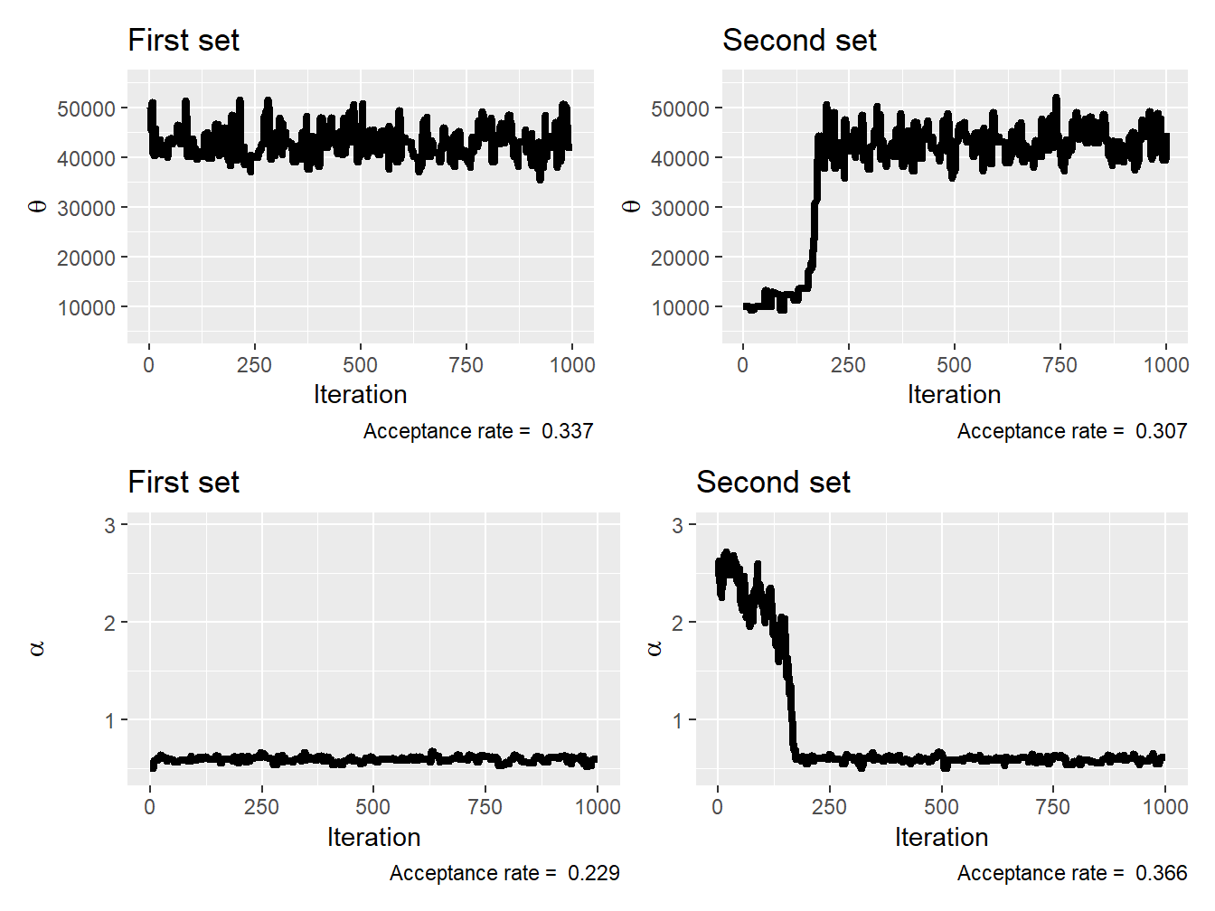
Example 9.4.3. Impact of Initial Parameters. Consider the motorcycle insurance data from Wasa used in Example 9.4.1. We wish to model the claim amount from motorcycle losses with a gamma distribution; that is,

\[ f_{X_i\,|\,\Theta = \theta,\, A = \alpha}(x_i) = \frac{1}{\theta^{\alpha}\Gamma(\alpha)} x_i^{\alpha-1} e^{-\frac{x_i}{\theta}}, \]

where $x_i$ is the $i^{\text{th}}$ claim amount. We assume that the prior distributions for both $\theta$ and $\alpha$ are noninformative and flat; that is,

\[ f_{\Theta , A}( \theta,\alpha) \propto 1, \quad \theta \in [0,\infty], \quad \alpha \in [0,\infty]. \]

Find the posterior distribution of the parameter using 1,000 iterations of the Metropolis–Hastings sampler. Use a normal proposal with a proposal variance $5 \times 10^7$ for $\theta$ and $1 \times 10^{-2}$ for $\alpha$, and rely on $\theta^{(0)} = 50,000$ and $\alpha^{(0)} = 0.5$ to start the Metropolis–Hastings sampler. Redo the experiment with $\theta^{(0)} = 10,000$ and $\alpha^{(0)} = 2.5$.

Show Example Solution

Solution. Starting from the the likelihood function and the prior distribution, we have that

\[ h(\theta,\alpha) \propto \prod_{i=1}^N \frac{1}{\theta^{\alpha}\Gamma(\alpha)} x_i^{\alpha-1} e^{-\frac{x_i}{\theta}}. \]

dataOhlsson <- dataOhlsson[dataOhlsson$skadkost > 0, ]
x <- dataOhlsson$skadkost
M <- 1000

set.seed(1)
sigma2theta <- 50000000
sigma2alpha <- 0.01

# First set of initial values
thetas1 <- rep(NA, M + 1)
thetas1[1] <- 50000
alphas1 <- rep(NA, M + 1)
alphas1[1] <- 0.5

accepttheta1 <- rep(NA, M)
acceptalpha1 <- rep(NA, M)

for (m in 2:(M + 1)) {
    # Let us start with theta and compute the logarithm of h for the past value
    loghpast <- sum(dgamma(x, scale = thetas1[m - 1], shape = alphas1[m - 1], log = TRUE))

    # Generate proposed parameter and compute logarithm of h for proposed value
    thetastar <- rnorm(1, mean = thetas1[m - 1], sd = sqrt(sigma2theta))
    if (thetastar > 0) {
        loghstar <- sum(dgamma(x, scale = thetastar, shape = alphas1[m - 1], log = TRUE))
    } else {
        loghstar <- -Inf
    }

    # Compute acceptance probability and copy new parameter value
    alphatheta <- exp(loghstar - loghpast)
    if (alphatheta > runif(1, min = 0, max = 1)) {
        thetas1[m] <- thetastar
        accepttheta1[m - 1] <- 1
    } else {
        thetas1[m] <- thetas1[m - 1]
        accepttheta1[m - 1] <- 0
    }

    # And then deal with alpha and compute the logarithm of h for the past
    # value
    loghpast <- sum(dgamma(x, scale = thetas1[m], shape = alphas1[m - 1], log = TRUE))

    # Generate proposed parameter and compute logarithm of h for proposed value
    alphastar <- rnorm(1, mean = alphas1[m - 1], sd = sqrt(sigma2alpha))
    if (thetastar > 0) {
        loghstar <- sum(dgamma(x, scale = thetas1[m], shape = alphastar, log = TRUE))
    } else {
        loghstar <- -Inf
    }

    # Compute acceptance probability and copy new parameter value
    alphaalpha <- exp(loghstar - loghpast)
    if (alphaalpha > runif(1, min = 0, max = 1)) {
        alphas1[m] <- alphastar
        acceptalpha1[m - 1] <- 1
    } else {
        alphas1[m] <- alphas1[m - 1]
        acceptalpha1[m - 1] <- 0
    }
}

# Second set of initial values
set.seed(1)
thetas2 <- rep(NA, M + 1)
thetas2[1] <- 10000
alphas2 <- rep(NA, M + 1)
alphas2[1] <- 2.5

accepttheta2 <- rep(NA, M)
acceptalpha2 <- rep(NA, M)

for (m in 2:(M + 1)) {
    # Let us start with theta and compute the logarithm of h for the past value
    loghpast <- sum(dgamma(x, scale = thetas2[m - 1], shape = alphas2[m - 1], log = TRUE))

    # Generate proposed parameter and compute logarithm of h for proposed value
    thetastar <- rnorm(1, mean = thetas2[m - 1], sd = sqrt(sigma2theta))
    if (thetastar > 0) {
        loghstar <- sum(dgamma(x, scale = thetastar, shape = alphas2[m - 1], log = TRUE))
    } else {
        loghstar <- -Inf
    }

    # Compute acceptance probability and copy new parameter value
    alphatheta <- exp(loghstar - loghpast)
    if (alphatheta > runif(1, min = 0, max = 1)) {
        thetas2[m] <- thetastar
        accepttheta2[m - 1] <- 1
    } else {
        thetas2[m] <- thetas2[m - 1]
        accepttheta2[m - 1] <- 0
    }

    # And then deal with alpha and compute the logarithm of h for the past
    # value
    loghpast <- sum(dgamma(x, scale = thetas1[m], shape = alphas2[m - 1], log = TRUE))

    # Generate proposed parameter and compute logarithm of h for proposed value
    alphastar <- rnorm(1, mean = alphas2[m - 1], sd = sqrt(sigma2alpha))
    if (thetastar > 0) {
        loghstar <- sum(dgamma(x, scale = thetas2[m], shape = alphastar, log = TRUE))
    } else {
        loghstar <- -Inf
    }

    # Compute acceptance probability and copy new parameter value
    alphaalpha <- exp(loghstar - loghpast)
    if (alphaalpha > runif(1, min = 0, max = 1)) {
        alphas2[m] <- alphastar
        acceptalpha2[m - 1] <- 1
    } else {
        alphas2[m] <- alphas2[m - 1]
        acceptalpha2[m - 1] <- 0
    }
}

$Trace plots based on two different starting parameter sets: $\theta^{(0)} = 50,000$ and $\alpha^{(0)} = 0.5$ (left panels), and $\theta^{(0)} = 10,000$ and $\alpha^{(0)} = 2.5$ (right panels)$

Figure 9.17: Trace plots based on two different starting parameter sets: $\theta^{(0)} = 50,000$ and $\alpha^{(0)} = 0.5$ (left panels), and $\theta^{(0)} = 10,000$ and $\alpha^{(0)} = 2.5$ (right panels)

Clearly, from Figure 9.17, the initial parameter value matters: for the first set, the starting value is close to the posterior mode, meaning that the final sample does not depend much on the starting value. For the second set, on the other hand, it takes about 200 iterations to get closer to where most of the density resides. Having a burn-in in the case of Metropolis–Hastings sampler is therefore a good idea to reduce the impact of initial guesses on the final posterior distribution.

In the next subsection, we learn a few methods and metrics to diagnose the convergence of the Markov chains generated via MCMC methods.

9.4.4 Markov Chain Diagnostics

There are many different tuning parameters in MCMC schemes, and they all have an impact on the convergence of the Markov chains generated by these methods. To understand the impact of these choices on the chains (e.g., number of iterations, length of burn-in, proposal distribution), we introduce a few methods to analyze their convergence.

9.4.4.1 Examining Trace Plots and Autocorrelation

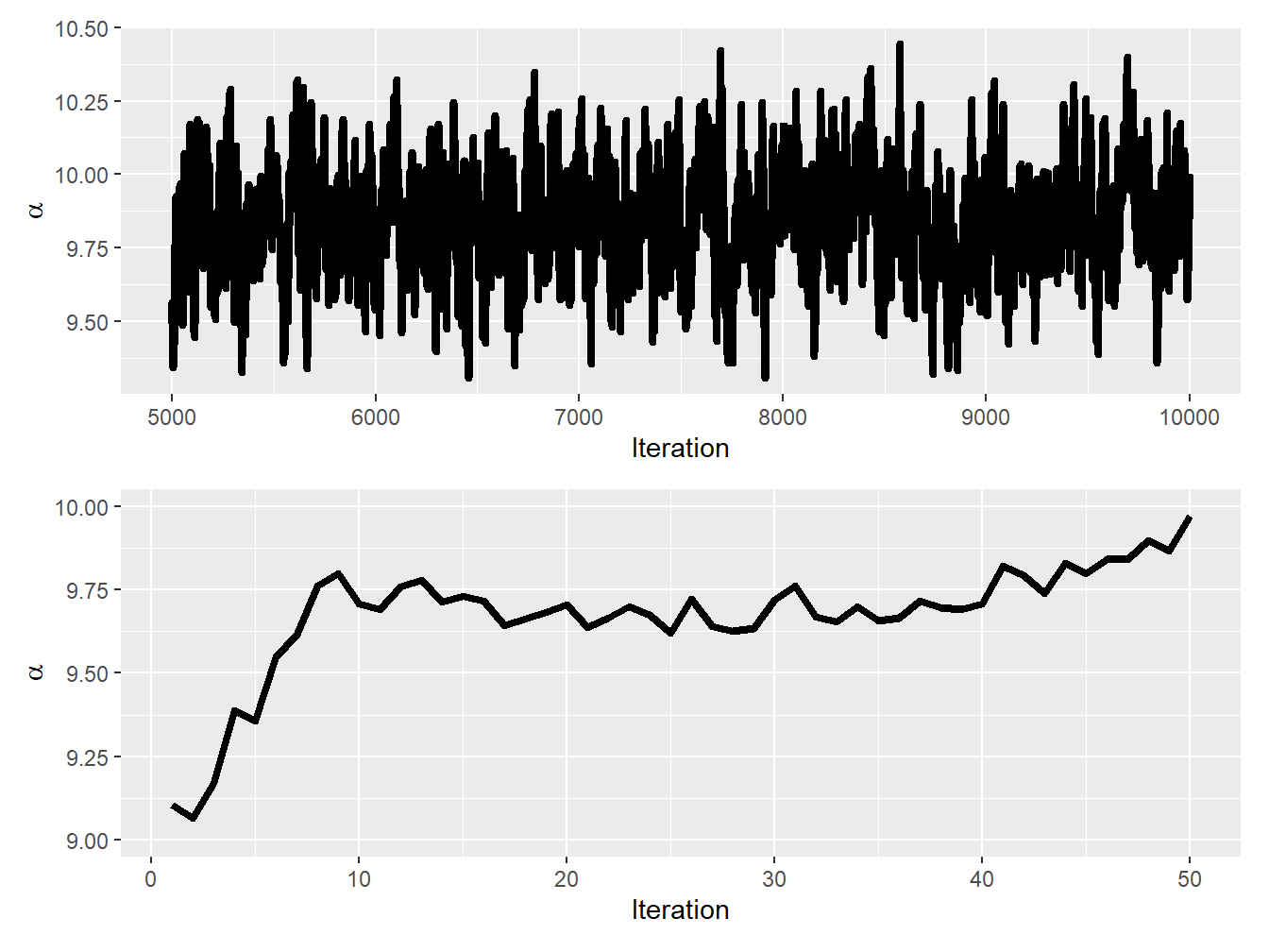
Trace Plot. The most elementary tool to assess whether MCMC chains have converged to the posterior distribution is the trace plot. As mentioned above, a trace plot displays the sequence of samples as a function of the iteration number, with the sample value on the $y$-axis and the iteration number on the $x$-axis. If the chain has converged, the trace plot should show a stable sequence of samples around the true posterior distribution that looks like a hairy caterpillar. However, if the chain has not yet converged, the trace plot may show a sequence of samples that still appear to be changing or have not yet settled into a stable pattern.

In addition to assessing convergence, trace plots can also be used to diagnose potential problems with MCMC algorithms, such as poor mixing or autocorrelation. For example, if the trace plot shows long periods of no change followed by abrupt jumps, this may indicate poor mixing and suggest that the MCMC algorithm needs to be adjusted or a different method should be used.

Lag-1 Autocorrelation. Another quantity that might be helpful is the lag-1 autocorrelation—the correlation between consecutive samples in a given chain:

\[ \mathrm{Cov}\left[ \theta_i^{(m)}, \theta_i^{(m-1)} \right]. \]

Note that if the autocorrelation is too high, it can indicate that the chain is not mixing well and is not sampling the posterior distribution effectively. This can result in poor convergence, longer run times, and decreased precision of the estimates obtained from the MCMC algorithm.

In addition to examining trace plots and computing autocorrelation coefficients, we can use other, more formal tools to evaluate whether the chains obtained are reliable and have converged.

9.4.4.2 Comparing Parallel Chains

Gelman–Rubin Statistic Another way to assess convergence is to run multiple chains in parallel from different starting points and check if their behavior is similar. In addition to comparing their trace plots, the chains can be compared by using a statistical test—the Gelman–Rubin test of Gelman and Rubin (1992). The latter test compares the within-chain variance to the between-chain variance; to calculate the statistic, we need to generate a small number of chains (say, $R$), each for $M-M^*$ post-burn-in iterations.

If the chains have converged, the within-chain variance should be similar to the between-chain variance. Assuming the parameter of interest is $\theta_i$, the within-chain variance is

\[ W = \frac{1}{R(M-M^*-1)} \sum_{r=1}^R \sum_{m=M^*+1}^{M} \left( \theta_{i,r}^{(m)} - \overline{\theta}_{i,r} \right)^2 , \]

where $\theta_{i,r}^{(m)}$ is the $m^{\text{th}}$ draw of $\theta_i$ in the $r^{\text{th}}$ chain and $\overline{\theta}_{i,r}$ is the sample mean of $\theta_i$ for the $r^{\text{th}}$ chain. The between-chain variance is given by

\[ B = \frac{M-M^*}{R-1} \sum_{r=1}^R \left( \overline{\theta}_{i,r} - \overline{\theta}_{i} \right), \]

where $\overline{\theta}_{i}$ is the overall sample mean of $\theta_i$ from all chains. The Gelman–Rubin statistic is

\[ \sqrt{\left( \frac{M-M^*-1}{M-M^*} + \frac{R+1}{R(M-M^*)} \frac{B}{W} \right) \frac{\text{df}}{\text{df}-2} }, \]

where $\text{df}$ is the degrees of freedom from Student’s $t$-distribution that approximates the posterior distribution. The statistic should produce a value close to 1 if the chain has converged. On the other hand, if the statistic value is greater than 1.1 or 1.2, this indicates that the chains may not have converged, and further analysis may be needed to determine why the chains are not mixing well.

9.4.4.3 Calculating Effective Sample Sizes

Effective Sample Size The effective sample size (ESS) is a measure of the number of independent samples obtained from an MCMC chain. Recall that in an MCMC chain, each sample is correlated with the previous sample; as a result, the effective number of independent samples is usually much smaller than the total number of samples generated by the MCMC algorithm. The ESS takes this correlation into account and provides an estimate of the number of independent samples that are equivalent to the correlated samples in the chain.

In general, a higher effective sample size indicates that the MCMC algorithm has produced more independent samples and is more likely to have accurately sampled the posterior distribution. A lower effective sample size, on the other hand, suggests that the MCMC algorithm may require further tuning or optimization to produce reliable posterior estimates.

The function multiESSof the R package mcmcse contains a function that gives the ESS of a multivariate Markov chain as described in Vats, Flegal, and Jones (2019). The package also includes an estimate of the minimum ESS required for a specified relative tolerance level (see function minESS).

We now apply these various diagnostics to an example.

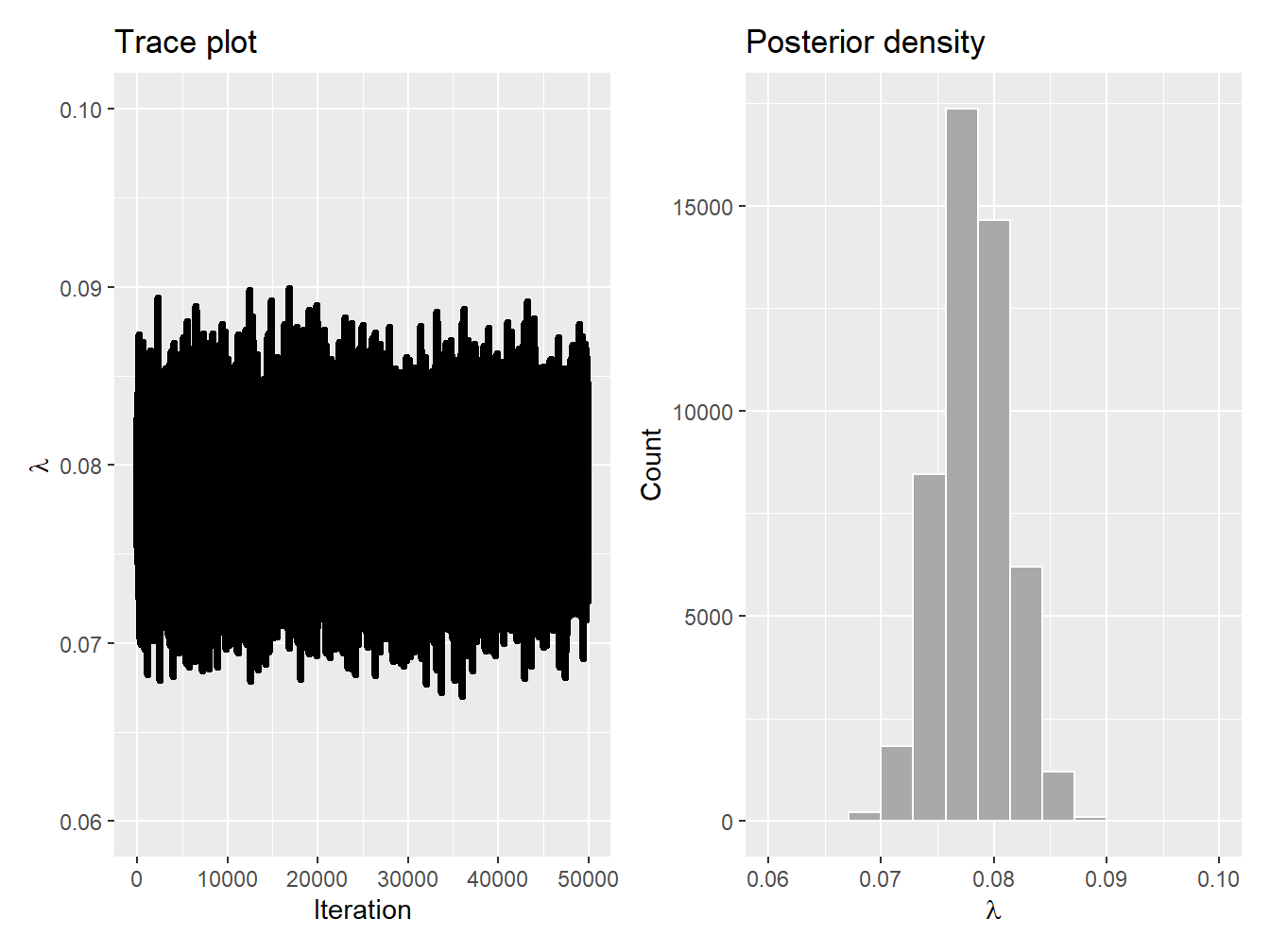
Example 9.4.4. Markov Chain Diagnostics. Consider the setup of Example 9.4.2. Using chains of 51,000 iterations and a burn-in of 1,000 iterations, calculate the various Markov chain diagnostics mentioned above.

Show Example Solution

Solution. Let us begin by generating five chains.

M <- 51000
Mstar <- 1000
R <- 5

set.seed(1)
delta2 <- 0.0001

lambdas <- matrix(data = NA, ncol = M + 1, nrow = R)
accept <- matrix(data = NA, ncol = M, nrow = R)

for (r in 1:R) {
    lambdas[r, 1] <- max(0.000001, mean(sgautonb$Clm_Count) + rnorm(1, mean = 0,
        sd = 0.1))

    for (m in 2:(M + 1)) {
        # Compute logarithm of h for past value
        loghpast <- sum(dpois(sgautonb$Clm_Count, lambda = lambdas[r, m - 1], log = TRUE))

        # Generate proposed parameter and compute logarithm of h for proposed
        # value
        lambdastar <- rnorm(1, mean = lambdas[r, m - 1], sd = sqrt(delta2))
        if (lambdastar > 0) {
            loghstar <- sum(dpois(sgautonb$Clm_Count, lambda = lambdastar, log = TRUE))
        } else {
            loghstar <- -Inf
        }

        # Compute acceptance probability and copy new parameter value
        alpha <- exp(loghstar - loghpast)
        if (alpha > runif(1, min = 0, max = 1)) {
            lambdas[r, m] <- lambdastar
            accept[r, m - 1] <- 1
        } else {
            lambdas[r, m] <- lambdas[r, m - 1]
            accept[r, m - 1] <- 0
        }
    }
}

Figure 9.18 reports the trace plot for the first chain: it indeed looks like a hairy caterpillar, which is a good sign.

$Trace plot for parameter $\lambda$$

Figure 9.18: Trace plot for parameter $\lambda$

autocorr <- acf(lambdas[1, (Mstar + 1):M], lag.max = 1, plot = FALSE)
cat("The lag-1 autocorrelation coefficient is", autocorr$acf[2])

The lag-1 autocorrelation coefficient is 0.651510865

The autocorrelation is also mild at 65%, again pointing towards good convergence behavior.

W <- 0
B <- 0
for (r in 1:R) {
    W <- W + 1/(R * (M - Mstar - 1)) * sum((lambdas[r, (Mstar + 1):M] - mean(lambdas[r,
        (Mstar + 1):M]))^2)
    B <- B + (M - Mstar)/(R - 1) * sum((mean(lambdas[r, (Mstar + 1):M]) - mean(lambdas[,
        (Mstar + 1):M]))^2)
}
# Assuming that df/(df-2) tends to 1
GR <- sqrt((M - Mstar - 1)/(M - Mstar) + (R + 1)/(R * (M - Mstar)) * B/W)
cat("The Gelman-Rubin statistic is", GR)

The Gelman-Rubin statistic is 1.00012696

The Gelman–Rubin statistic is very close to 1 in this case, meaning that the chains converged.

library("mcmcse")
ess <- multiESS(matrix(lambdas[1, ]))
mess <- minESS(p = 1)
cat("The ESS is", ess, "and the minimum ESS is", mess)

The ESS is 9927.29934 and the minimum ESS is 6146

The last diagnostic refers to the ESS, and its comparison to the minimum ESS. In our case, the ESS is about 9,927, and the minimum ESS is 6,146. Since our ESS is above the minimum, we know we have a large enough sample to adequately capture the posterior distribution of $\lambda$.

9.5 Bayesian Statistics in Practice

In Section 9.5, you learn how to:

Describe the main computing resources available for Bayesian statistics and modeling.
Apply one of them to loss data.

Fortunately for end users, some of these methods are readily available in R, meaning that they are quite accessible. Some popular computing resources used in Bayesian statistics are listed below:

RSTAN, named in honor of Stanislaw Ulam, is an R implementation of the widely used STAN probabilistic programming language for Bayesian statistical modeling and inference. It is highly flexible and allows users to define complex statistical models.
nimble stands for Numerical Inference for Bayesian and Likelihood Estimation and is an R package designed for statistical computing and hierarchical modeling. nimble provides a high-level programming language that allows users to define complex statistical models with ease.
R2OpenBUGS allows R users to use OpenBUGS, a classic and widely-used software package for Bayesian data analysis. It uses MCMC techniques like Gibbs sampling to obtain samples from the posterior distribution.
rjags is an R implementation of the JAGS (Just Another Gibbs Sampler) program. It is an open-source software that was developed as an extension of BUGS. It provides a platform-independent engine for the BUGS language, allowing for the use of BUGS models in various environments. Like BUGS, JAGS is also used for Bayesian analysis through MCMC sampling techniques.

In what follows, we will use the nimble package in the context of loss data.

Example 9.5.1. The nimble package. Similar to the setup of Example 9.4.2, consider that each policyholder’s claim count (frequency) is distributed as a Poisson random variable such that \[ p_{N_i\,|\,\Lambda=\lambda}(n_i) = \frac{\lambda^{n_i}e^{-\lambda}}{n_i!}, \] where $n_i$ is the number of claims associated with the $i^{\text{th}}$ policyholder. Unlike the previous example, however, let us assume an inverse gamma prior with a shape parameter of 2 and a scale parameter of 5.²⁴

Find the posterior distribution of the parameter by creating a chain of 51,000 iterations and a burn-in of 1,000 iterations using the nimble package.

Show Example Solution

Solution. First, we need to define the model using the nimble language. Simply put, the model is comprised of a likelihood density and a prior density. The former links the observations to a Poisson distribution with parameter $\lambda$, and the latter states the prior distribution, which is inverse gamma with shape and scale parameters of 2 and 5, respectively.

claimmodel <- nimbleCode({
    for (i in 1:N) {
        # Likelihood
        count[i] ~ dpois(lambda)
    }
    # Prior distribution
    lambda ~ dinvgamma(shape = 2, scale = 5)
})

Then, we define the data, the constant (i.e., the number of observations in this case), the parameter list (i.e., only $\lambda$ here), and the initial value set to 0.05 in this illustration.

claimdata <- list(count = sgautonb$Clm_Count)
claimconstant <- list(N = length(sgautonb$Clm_Count))
claimparameters <- c("lambda")
claiminitial <- list(lambda = 0.05)

The MCMC chain is then run using for 51,000 iterations and a burn-in of 1,000 iterations.

mcmcoutput <- nimbleMCMC(code = claimmodel, data = claimdata, constants = claimconstant,
    inits = claiminitial, monitors = claimparameters, niter = 51000, nburnin = 1000,
    nchains = 1)

Finally, we display the trace plot, obtain the histogram of the posterior distribution of $\lambda$, and compute some descriptive statistics of the parameter.

$Trace plot and posterior density for parameter $\lambda$$

Figure 9.19: Trace plot and posterior density for parameter $\lambda$

The posterior mean of the parameter is 0.0781913941

The posterior standard deviation of the parameter is 0.00309462947

This simple illustration demonstrates the simplicity of utilizing R packages to generate MCMC chains, all without the need for writing extensive code. For more details on the nimble package, see Valpine et al. (2017).

9.6 Further Resources and Contributors

Many great books exist on Bayesian statistics and MCMC schemes. We refer the interested reader to Bernardo and Smith (2009) and Robert and Casella (1999) for an advanced treatment of these topics.

A number of academic articles in actuarial science relied on Bayesian statistics and MCMC schemes over the past 40 years; see, for instance, Heckman and Meyers (1983), Meyers and Schenker (1983), Cairns (2000), Cairns, Blake, and Dowd (2006), Hartman and Heaton (2011), Bermúdez and Karlis (2011), Hartman and Groendyke (2013), Fellingham, Kottas, and Hartman (2015), Bignozzi and Tsanakas (2016), Bégin (2019), Huang and Meng (2020), Bégin (2021), Cheung et al. (2021), and Bégin (2023).

Contributors

Jean-François Bégin, Simon Fraser University, is the principal author of the initial version of this chapter. Email: jbegin@sfu.ca for chapter comments and suggested improvements.
Chapter reviewers include: Brian Hartman, Chun Yong, Margie Rosenberg, and Gary Dean.

Bibliography

Bermúdez, Lluı́s, and Dimitris Karlis. 2011. “Bayesian Multivariate Poisson Models for Insurance Ratemaking.” Insurance: Mathematics and Economics 48 (2): 226–36.

Bernardo, José M, and Adrian FM Smith. 2009. Bayesian Theory. John Wiley & Sons: New York, NY, United States of America.

Bégin, Jean-François. 2019. “Economic Scenario Generator and Parameter Uncertainty: A Bayesian Approach.” ASTIN Bulletin 49 (2): 335–72.

———. 2021. “On Complex Economic Scenario Generators: Is Less More?” ASTIN Bulletin 51 (3): 779–812.

———. 2023. “Ensemble Economic Scenario Generators: Unity Makes Strength.” North American Actuarial Journal 27 (3): 444–71.

Bignozzi, Valeria, and Andreas Tsanakas. 2016. “Parameter Uncertainty and Residual Estimation Risk.” Journal of Risk and Insurance 83 (4): 949–78.

Cairns, Andrew JG. 2000. “A Discussion of Parameter and Model Uncertainty in Insurance.” Insurance: Mathematics and Economics 27 (3): 313–30.

Cairns, Andrew JG, David Blake, and Kevin Dowd. 2006. “A Two-Factor Model for Stochastic Mortality with Parameter Uncertainty: Theory and Calibration.” Journal of Risk and Insurance 73 (4): 687–718.

Cheung, Eric CK, Weihong Ni, Rosy Oh, and Jae-Kyung Woo. 2021. “Bayesian Credibility Under a Bivariate Prior on the Frequency and the Severity of Claims.” Insurance: Mathematics and Economics 100: 274–95.

Cowles, Mary Kathryn. 2013. Applied Bayesian Statistics: With R and OpenBUGS Examples. Springer Science & Business Media: New York, NY, United States of America.

Fellingham, Gilbert W, Athanasios Kottas, and Brian M Hartman. 2015. “Bayesian Nonparametric Predictive Modeling of Group Health Claims.” Insurance: Mathematics and Economics 60: 1–10.

Gelfand, Alan E, and Adrian FM Smith. 1990. “Sampling-Based Approaches to Calculating Marginal Densities.” Journal of the American Statistical Association 85 (410): 398–409.

Gelman, Andrew, and Donald B Rubin. 1992. “Inference from Iterative Simulation Using Multiple Sequences.” Statistical Science, 457–72.

Hartman, Brian M, and Chris Groendyke. 2013. “Model Selection and Averaging in Financial Risk Management.” North American Actuarial Journal 17 (3): 216–28.

Hartman, Brian M, and Matthew J Heaton. 2011. “Accounting for Regime and Parameter Uncertainty in Regime-Switching Models.” Insurance: Mathematics and Economics 49 (3): 429–37.

Hastings, WK. 1970. “Monte Carlo Sampling Methods Using Markov Chains and Their Applications.” Biometrika 57 (1): 97–109.

Haueter, Niels Viggo. 2017. “A History of UK Insurance.” Swiss Re Corporate History: Zurich, Switzerland.

Heckman, Philip E, and Glenn G Meyers. 1983. “The Calculation of Aggregate Loss Distributions from Claim Severity and Claim Count Distributions.” In Proceedings of the Casualty Actuarial Society, 70:49–66. 133-134.

Huang, Yifan, and Shengwang Meng. 2020. “A Bayesian Nonparametric Model and Its Application in Insurance Loss Prediction.” Insurance: Mathematics and Economics 93: 84–94.

Metropolis, Nicholas, Arianna W Rosenbluth, Marshall N Rosenbluth, Augusta H Teller, and Edward Teller. 1953. “Equation of State Calculations by Fast Computing Machines.” Journal of Chemical Physics 21 (6): 1087–92.

Meyers, Glenn. 1994. “Quantifying the Uncertainty in Claim Severity Estimates for an Excess Layer When Using the Single Parameter Pareto.” In Proceedings of the Casualty Actuarial Society, 81:91–122.

Meyers, Glenn, and Nathaniel Schenker. 1983. “Parameter Uncertainty in the Collective Risk Model.” PCAS LXX 111: 15.

O’Donnell, Terence. 1936. History of Life Insurance in Its Formative Years. American Conservation Company: Chicago, IL, United States of America.

Robert, Christian P, and George Casella. 1999. Monte Carlo Statistical Methods. Springer: New York, NY, United States of America.

Valpine, Perry de, Daniel Turek, Christopher J Paciorek, Clifford Anderson-Bergman, Duncan Temple Lang, and Rastislav Bodik. 2017. “Programming with Models: Writing Statistical Algorithms for General Model Structures with nimble.” Journal of Computational and Graphical Statistics 26 (2): 403–13.

Vats, Dootika, James M Flegal, and Galin L Jones. 2019. “Multivariate Output Analysis for Markov Chain Monte Carlo.” Biometrika 106 (2): 321–37.

Wolny-Dominiak, Alicja, and Michal Trzesiok. 2014. “Package ‘insuranceData’.” The Comprehensive R Archive Network.

Each coin toss can be seen as a Bernoulli random variable, meaning that their sum is a binomial with parameters $q=0.5$ and $m=5$. See Chapter 20.1 for more details.↩︎
Specifically, we use a uniform over $[0,1]$ for our prior distribution. As explained in Section 9.2.3, this type of prior is said to be noninformative.↩︎
This is also an application of the beta–binomial conjugate family that will be explained in Section 9.3.1 ↩︎
There is also a rich history blending prior information with data in loss modeling and in actuarial science, generally speaking; it is known as credibility. In technical terms, credibility theory’s main challenge lies in identifying the optimal linear approximation to the mean of the Bayesian predictive density. This is the reason credibility theory shares numerous outcomes with both linear filtering and the broader field of Bayesian statistics. For more details on experience rating using credibility theory, see Chapter 12.↩︎
This question was adapted from the Be An Actuary website. See here for more details.↩︎
The law of total probability states that the total probability of an event $B$ is equal to the sum of the probabilities of $B$ occurring under different conditions, weighted by the probabilities of those conditions. In the case where there are only two different conditions (let us say $A$ and $A^{\text{c}}$), we simply need to consider these two conditions. In all generality, however, we would need to consider more possibilities if the sample space cannot be divided into only two events.↩︎
This question was taken from the Society of Actuaries Sample Questions for Exam P. See here for more details.↩︎
The data are from the General Insurance Association of Singapore, an organization consisting of non-life insurers in Singapore. These data contain the number of car accidents for $n=7{,}483$ auto insurance policies with several categorical explanatory variables and the exposure for each policy.↩︎
For the sake of simplicity, we only consider one parameter in our derivation here. Note that, later, we will consider cases with more than one parameter and that this extension does not change the bulk of our results and derivations.↩︎
This question is a modified version of Sample Question 184 of the Society of Actuaries Exam C sample questions.↩︎
Here, we assume that the domain of the beta is $[0,1]$, meaning that $\theta = 1$. For more details, see Chapter 20.↩︎
This question is Sample Question 5 of the Society of Actuaries Exam C sample questions.↩︎
Conjugate families for the normal distribution with unknown $\sigma^2$ can also be derived. For the sake of simplicity, we will only focus on the case with known variance parameter in this book.↩︎
For an overview of the theory behind MCMC methods, see Robert and Casella (1999).↩︎
The Gibbs sampler can be seen as a special case of the more general Metropolis–Hastings algorithm. Specifically, with Gibbs’ method, all proposals are automatically accepted; that is, $\alpha\left(\theta_1^{(0)},\theta_1^*\right)=1$.↩︎
Note that the inverse gamma prior combined with a Poisson distribution does not generally lead to closed-form posterior densities and thus requires us to use MCMC methods.↩︎