Chapter 16 Quantifying Dependence
Chapter Preview. Dependence modeling involves using statistical models to describe the dependence structure between random variables and enables us to understand the relationships between variables in a dataset. This chapter introduces readers to techniques for modeling and quantifying dependence or association of multivariate distributions. Section 16.1 elaborates basic measures for modeling the dependence between variables.
Section 16.2 introduces an approach to modeling dependence using copulas which is reinforced with practical illustrations in Section 16.3. The types of copula families and basic properties of copula functions are explained in Section 16.4. The chapter concludes by explaining why the study of dependence modeling is important in Section 16.6.
16.1 Classic Measures of Scalar Associations
In this section, you learn how to:
- Estimate correlation using the Pearson method
- Use rank based measures like Spearman, Kendall to estimate correlation
- Measure tail dependency
In this chapter, we consider the first two variables from an insurance dataset of sample size (\(n = 1500\)) introduced in Frees and Valdez (1998) and is now readily available in the copula package; losses and expenses.
- \({\tt LOSS}\), general liability claims from the Insurance Services Office, Inc. (ISO)
- \({\tt ALAE}\), specifically attributable to the settlement of individual claims (e.g. lawyer’s fees, claims investigation expenses)
We would like to know whether the distribution of \({\tt LOSS}\) depends on the distribution of \({\tt ALAE}\) or whether they are statistically independent. To visualize the relationship between losses and expenses, the scatterplots in Figure 16.1 are created on dollar and log dollar scales. It is difficult to see any relationship between the two variables in the left-hand panel. Their dependence is more evident when viewed on the log scale, as in the right-hand panel. This section elaborates basic measures for modeling the dependence between variables.
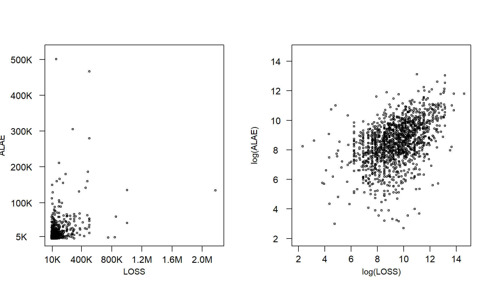
Figure 16.1: Scatter Plot of LOSS and ALAE
R Code for Loss versus Expense Scatterplots
16.1.1 Association Measures for Quantitative Variables
For this section, consider a pair of random variables \((X,Y)\) having joint distribution function \(F(\cdot)\) and a random sample \((X_i,Y_i), i=1, \ldots, n\). For the continuous case, suppose that \(F(\cdot)\) has absolutely continuous marginals with marginal density functions.
16.1.1.1 Pearson Correlation
Define the sample covariance function \(\widehat{Cov}(X,Y) = \frac{1}{n} \sum_{i=1}^n (X_i - \bar{X})(Y_i - \bar{Y})\), where \(\bar{X}\) and \(\bar{Y}\) are the sample means of \(X\) and \(Y\), respectively. Then, the product-moment (Pearson) correlationPearson correlation, a measure of the linear correlation between two variables can be written as
\[ r = \frac{\widehat{Cov}(X,Y)}{\sqrt{\widehat{Cov}(X,X)\widehat{Cov}(Y,Y)}} = \frac{\widehat{Cov}(X,Y)}{\sqrt{\widehat{Var}(X)}\sqrt{\widehat{Var}(Y)}}. \]
The correlation statistic \(r\) is widely used to capture linear association between random variables. It is a (nonparametric) estimator of the correlation parameter \(\rho\), defined to be the covariance divided by the product of standard deviations.
This statistic has several important features. Unlike regression estimators, it is symmetric between random variables, so the correlation between \(X\) and \(Y\) equals the correlation between \(Y\) and \(X\). It is unchanged by linear transformations of random variables (up to sign changes) so that we can multiply random variables or add constants as is helpful for interpretation. The range of the statistic is \([-1,1]\) which does not depend on the distribution of either \(X\) or \(Y\).
Further, in the case of independence, the correlation coefficient \(r\) is 0. However, it is well known that zero correlation does not in general imply independence, one exception is the case of normally distributed random variables. The correlation statistic \(r\) is also a (maximum likelihood) estimator of the association parameter for the bivariate normal distribution. So, for normally distributed data, the correlation statistic \(r\) can be used to assess independence. For additional interpretations of this well-known statistic, readers will enjoy Lee Rodgers and Nicewander (1998).
You can obtain the Pearson correlationA measure of the linear correlation between two variables statistic \(r\) using the cor() function in R and selecting the pearson method. This is demonstrated below by using the \({\tt LOSS}\) rating variable in millions of dollars and \({\tt ALAE}\) amount variable in dollars from the dataset in Figure 16.1.
R Code for Pearson Correlation Statistic
From the R output above, \(r=0.4\), which indicates a positive association between \({\tt LOSS}\) and \({\tt ALAE}\). This means that as the loss amount of a claim increases we expect expenses to increase.
16.1.2 Rank Based Measures
16.1.2.1 Spearman’s Rho
The Pearson correlation coefficient does have the drawback that it is not invariant to nonlinear transforms of the data. For example, the correlation between \(X\) and \(\log Y\) can be quite different from the correlation between \(X\) and \(Y\). As we see from the R code for the Pearson correlation statistic above, the correlation statistic \(r\) between the \({\tt ALAE}\) variable in logarithmic dollars and the \({\tt LOSS}\) amounts variable in dollars is \(0.33\) as compared to \(0.4\) when we calculate the correlation between the \({\tt ALAE}\) variable in dollars and the \({\tt LOSS}\) amounts variable in dollars. This limitation is one reason for considering alternative statistics.
Alternative measures of correlation are based on ranks of the data. Let \(R(X_j)\) denote the rank of \(X_j\) from the sample \(X_1, \ldots, X_n\) and similarly for \(R(Y_j)\). Let \(R(X) = \left(R(X_1), \ldots, R(X_n)\right)'\) denote the vector of ranks, and similarly for \(R(Y)\). For example, if \(n=3\) and \(X=(24, 13, 109)\), then \(R(X)=(2,1,3)\). A comprehensive introduction of rank statistics can be found in, for example, Hettmansperger (1984). Also, ranks can be used to obtain the empirical distribution function, refer to Section 4.4.1 for more on the empirical distribution function.
With this, the correlation measure of Spearman (1904) is simply the product-moment correlation computed on the ranks:
\[ r_S = \frac{\widehat{Cov}(R(X),R(Y))}{\sqrt{\widehat{Cov}(R(X),R(X))\widehat{Cov}(R(Y),R(Y))}} = \frac{\widehat{Cov}(R(X),R(Y))}{(n^2-1)/12} . \]
You can obtain the Spearman correlation statistic \(r_S\) using the cor() function in R and selecting the spearman method. From below, the Spearman correlation between the \({\tt LOSS}\) variable and \({\tt ALAE}\) variable is \(0.45\).
R Code for Spearman Correlation Statistic
We can show that the Spearman correlation statistic is invariant under strictly increasing transformations. From the R Code for the Spearman correlation statistic above, \(r_S=0.45\) between the \({\tt ALAE}\) variable in logarithmic dollars and \({\tt LOSS}\) amount variable in dollars.
Example 16.1.1. Calculation by Hand.
You are given the following six observations:
\[\begin{array}{|c|c|c|} \hline \textbf{Observation} & x \textbf{ value} & y \textbf{ value}\\ \hline 1 & 15 & 19 \\ \hline 2 & 9 & 7 \\ \hline 3 & 5 & 13 \\ \hline 4 & 3 & 15 \\ \hline 5 & 21 & 17 \\ \hline 6 & 12 & 11 \\ \hline \end{array}\]
Calculate the sample Spearman’s \(\rho\).
Show Example Solution
16.1.2.2 Kendall’s Tau
An alternative measure that uses ranks is based on the concept of concordance. An observation pair \((X,Y)\) is said to be concordantAn observation pair (x,y) is said to be concordant if the observation with a larger value of x has also the larger value of y (discordantAn observation pair (x,y) is said to be discordant if the observation with a larger value of x has the smaller value of y) if the observation with a larger value of \(X\) has also the larger (smaller) value of \(Y\). Then \(\Pr(concordance) = \Pr[ (X_1-X_2)(Y_1-Y_2) >0 ]\) , \(\Pr(discordance) = \Pr[ (X_1-X_2)(Y_1-Y_2) <0 ]\), \(\Pr(tie) = \Pr[ (X_1-X_2)(Y_1-Y_2) =0 ]\) and
\[ \begin{array}{rl} \tau(X,Y) &= \Pr(concordance) - \Pr(discordance) \\ & = 2\Pr(concordance) - 1 + \Pr(tie). \end{array} \]
To estimate this, the pairs \((X_i,Y_i)\) and \((X_j,Y_j)\) are said to be concordant if the product \(sgn(X_j-X_i)sgn(Y_j-Y_i)\) equals 1 and discordant if the product equals -1. Here, \(sgn(x)=1,0,-1\) as \(x>0\), \(x=0\), \(x<0\), respectively. With this, we can express the association measure of Maurice G. Kendall (1938), known as Kendall’s tau, as
\[ \begin{array}{rl} \hat{\tau} &= \frac{2}{n(n-1)} \sum_{i<j} ~sgn(X_j-X_i) \times sgn(Y_j-Y_i)\\ &= \frac{2}{n(n-1)} \sum_{i<j} ~sgn(R(X_j)-R(X_i)) \times sgn(R(Y_j)-R(Y_i)) . \end{array} \]
Interestingly, Hougaard (2000), page 137, attributes the original discovery of this statistic to Fechner (1897), noting that Kendall’s discovery was independent and more complete than the original work.
You can obtain Kendall’s tau using the cor() function in R and selecting the kendall method. From below, \(\hat{\tau}=0.32\) between the \({\tt LOSS}\) variable in dollars and the \({\tt ALAE}\) variable in dollars. When there are ties in the data, the cor() function computes Kendall’s tau_b as proposed by M. G. Kendall (1945).
R Code for Kendall’s Tau
Also, to show that the Kendall’s tau is invariant under strictly increasing transformations, we see that \(\hat{\tau}=0.32\) between the \({\tt ALAE}\) variable in logarithmic dollars and the \({\tt LOSS}\) amount variable in dollars.
Example 16.1.2. Calculation by Hand.
You are given the following six observations:
\[ \begin{array}{|c|c|c|} \hline \textbf{Observation} & x \textbf{ value} & y \textbf{ value}\\ \hline 1 & 15 & 19 \\ \hline 2 & 9 & 7 \\ \hline 3 & 5 & 13 \\ \hline 4 & 3 & 15 \\ \hline 5 & 21 & 17 \\ \hline 6 & 12 & 11 \\ \hline \end{array} \]
Calculate the sample Kendall’s \(\tau\).
Show Example Solution
16.1.3 Tail Dependence Coefficients
Tail dependence is a statistical concept that measures the strength of the dependence between two variables in the tails of their distribution. Specifically, tail dependence measures the correlation or dependence between the extreme values of two variables beyond a certain threshold, that is, the dependence in the corner of the lower-left quadrant or upper-right quadrant of the bivariate distribution. Tail dependence is essential in many areas of finance, economics, and risk management. For example, it is relevant in analyzing extreme events, such as financial crashes, natural disasters, and pandemics. In these situations, tail dependence can help to determine the likelihood of joint extreme events occurring and to develop strategies to manage the associated risks.
In Figure 16.2, the concept of tail dependence is demonstrated through an example. The figure showcases two randomly generated variables with a Kendall’s Tau of 0.7. On the left side of Figure 16.2, the variables (\(X\) and \(Y\)) are simulated using the bivariate normal distribution, while on the right side, they are generated using the bivariate t-distribution. Although both sides display a Kendall’s Tau of 0.7, there is a difference in the upper right quadrant (above the dashed lines) on each panel. In the left panel, the values in the upper right quadrant (upper tails of \(X\) and \(Y\)) are independent, while in the right panel, the upper tail values appear to be correlated (the upper right corners of the right panel contain 4 points). This suggests that the probability of \(Y\) occurring above a high threshold (e.g., the dashed line in the figure) when \(X\) exceeds the same threshold is higher in the right panel than in the left panel of Figure 16.2.
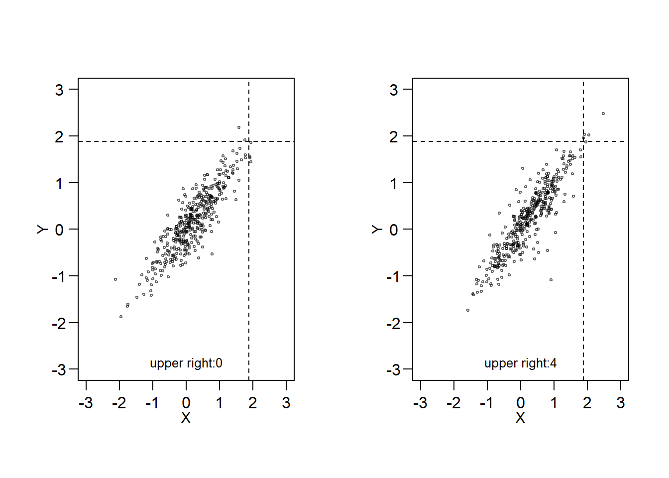
Figure 16.2: Left Panel: Upper tails of \(X\) and \(Y\) are independent. Right Panel: Upper tails of \(X\) and \(Y\) appear to be dependent.
Consider a pair of random variables \((X,Y)\), from definitions provided in Joe (1997), the upper tail dependent coefficient denoted by \(\lambda_{\text{up}}\) is given by:
\[ \lambda_\text{up} {=} \lim _{u \rightarrow 1^-} \mathrm{Pr}\left\{X>F_X^{-1}(u) \mid Y>F_Y^{-1}(u)\right\}, \] in case the limit exists. Here, \(F_X^{-1}(u)\) and \(F_Y^{-1}(u)\) denote the quantiles of \(X\) and \(Y\) at the level \(u\). Then, \(X\) and \(Y\) are said to be upper tail-dependent if \(\lambda_\text{up}\in(0,1]\) and upper tail-independent if \(\lambda_\text{up}=0\). When a variable reaches an extreme high value, the upper tail-dependent condition indicates that the other variable also reaches an extremely high value. On the other hand, the upper tail-independent suggests that the extreme values of the two variables are not related to each other. Similarly, the lower tail dependence coefficient, \(\lambda_{\text{lo}}\), is defined as:
\[ \lambda_{\text{lo}} {=} \lim _{u \rightarrow 0^+} \mathrm{Pr}\left\{X \leq F_X^{-1}(u) \mid Y \leq Y^{-1}(u)\right\} . \]
Let \(R(X_j)\) and \(R(Y_j)\) denote the rank of \(X_j\) and \(Y_j\), \(j=1,\ldots, n\), respectively. From Schmidt (2005), non-parametric estimates of \(\lambda_\text{up}\) and \(\lambda_\text{lo}\) are given by:
\[ \hat{\lambda}_{\text{lo}}=\frac{1}{k} \sum_{j=1}^n I\left\{R(X_j)\leq k, R(Y_j) \leq k\right\}, \] and
\[ \begin{aligned} \hat{\lambda}_{\text{up}} & =\frac{1}{k} \sum_{j=1}^n I\left\{R(X_j)>n-k, R(Y_j)>n-k\right\}, \end{aligned} \]
where \(k \in {1, . . .,n}\) is the threshold rank and a parameter to be chosen by the analyst, \(k=k(n) \rightarrow \infty \text { and } k / n \rightarrow 0 \text { as } n \rightarrow \infty \text {, }\). Here, \(n\) is the sample size, and \(I\{\cdot\}\) takes the value of 1 if the condition is satisfied, and 0 otherwise.
Figure 16.3 shows the scatter plot of the ranks of the \({\tt LOSS}\) variable and the \({\tt ALAE}\) variable. You can obtain the upper and lower tail dependent coefficient using the tdc() function from the FRAPO package in R. From below, \(\hat{\lambda}_{\text{up}}=0.39\), at \(k=75\) (note that \(n=1500\)), between the \({\tt LOSS}\) variable and the \({\tt ALAE}\) variable and \(\hat{\lambda}_{\text{lo}}=0.13\). The results implies the losses and expenses variables appear to be more upper-tailed dependent.
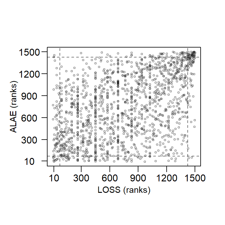
Figure 16.3: Scatter Plot of Ranks of LOSS and ALAE
R Code for Tail Dependence Coefficient
Show Quiz Solution
16.2 Introduction to Copulas
In this section, you learn how to:
- Describe a multivariate distribution function in terms of a copula function.
16.2.1 Definition of a Copula
Copulas are widely used in insurance and many other fields to model the dependence among multivariate outcomes as they expresses the dependence between the variables explicitly. Recall that the joint cumulative distribution function (\(cdf\)) for two variables \(Y_1\) and \(Y_2\) is given by:
\[ {F}(y_1, y_2)= {\Pr}(Y_1 \leq y_1, Y_2 \leq y_2) . \]
For the multivariate case in \(p\) dimensions, we have:
\[ {F}(y_1,\ldots, y_p)= {\Pr}(Y_1 \leq y_1,\ldots ,Y_p \leq y_p) . \]
The joint distribution considers both the marginal distributions and how the variables are related to each other. However, it expresses this dependence implicitly. Copulas offer a different method that allows us to break down the joint distribution of variables into individual components (the marginal distributions and a copula) that can be adjusted separately.
A copulaA multivariate distribution function with uniform marginals is a multivariate distribution function with uniform marginals. Specifically, let \(\{U_1, \ldots, U_p\}\) be \(p\) uniform random variables on \((0,1)\). Their distribution function \[{C}(u_1, \ldots, u_p) = \Pr(U_1 \leq u_1, \ldots, U_p \leq u_p),\]
is a copula. We seek to use copulas in applications that are based on more than just uniformly distributed data. Thus, consider arbitrary marginal distribution functions \({F}_1(y_1)\),…,\({F}_p(y_p)\). Then, we can define a multivariate distribution function using the copula such that
\[\begin{equation} {F}(y_1, \ldots, y_p)= {C}({F}_1(y_1), \ldots, {F}_p(y_p)). \tag{16.1} \end{equation}\]
Here, \(F\) is a multivariate distribution function, and the resulting value from the copula function is limited to a range of \([0,1]\) as it relates to probabilities. Sklar (1959) showed that \(any\) multivariate distribution function \(F\), can be written in the form of equation (16.1), that is, using a copula representation.
Sklar also showed that, if the marginal distributions are continuous, then there is a unique copula representation. Hence, copulas can be used instead of joint distribution functions. In order to be considered valid, they must meet the necessary requirements of a valid joint cumulative distribution function. In this chapter we focus on copula modeling with continuous variables. A copula \(C\) is considered to be absolutely continuous if the density
\[ c(u_1, \ldots, u_p)=\frac{\partial^p}{\partial_{u_p}\ldots \partial_{u_1}}C(u_1, \ldots, u_p), \]
exists. For the discrete case, readers can see Joe (2014) and Genest and Nešlohva (2007). For the bivariate case where \(p=2\), we can write a copula and the distribution function of two random variables as
\[ {C}(u_1, \, u_2) = \Pr(U_1 \leq u_1, \, U_2 \leq u_2) \]
and
\[ {F}(y_1, \, y_2)= {C}({F}_1(y_1), {F}_p(y_2)). \]
One example of a bivariate copula is the product copula, also called the independence copula, as it captures the property of independence of the two variables \(Y_1\) and \(Y_2\). The copula (distribution function) is
\[ {F}(y_1, \, y_2)= {C}({F}_1(y_1), {F}_p(y_2))={F}_1(y_1){F}_p(y_2)=u_1u_2=\Pi(u). \]
In Figure 16.4, both the distribution function and scatter plot of observations generated from the independence copula are displayed. The scatter plot indicates that there is no correlation between the two components, \(U_1\) and \(U_2\).
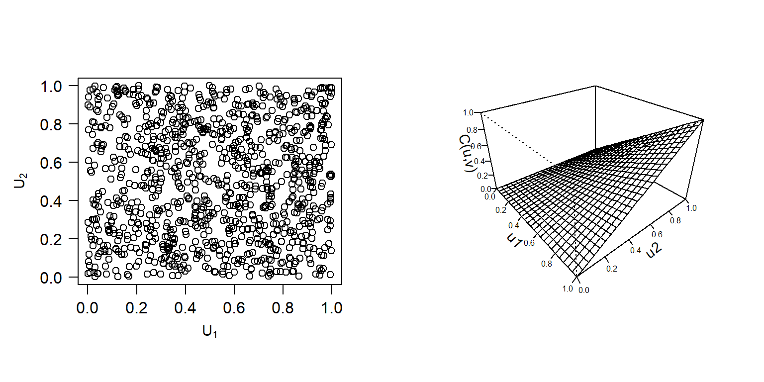
Figure 16.4: Left: Scatterplot of observations from Independence Copula. Right: Plot for distribution function for Independence Copula.
R Code for Independence Copula Plots
There is another type of copula that is frequently utilized, known as Frank’s Copula (Frank 1979). This copula can represent both positive and negative dependence and has a straightforward analytic structure. The copula (distribution function) is
\[\begin{equation} {C}(u_1,u_2) = \frac{1}{\gamma} \log \left( 1+ \frac{ (\exp(\gamma u_1) -1)(\exp(\gamma u_2) -1)} {\exp(\gamma) -1} \right). \tag{16.2} \end{equation}\]
This is a bivariate distribution function with its domain on the unit square \([0,1]^2.\) Here \(\gamma\) is the dependence parameter, that is, the range of dependence is controlled by the parameter \(\gamma\). Positive association increases as \(\gamma\) increases. As we will see, this positive association can be summarized with Spearman’s rho (\(\rho_S\)) and Kendall’s tau (\(\tau\)).
In Figure 16.5, we can see scatterplots of data generated from the Frank’s copula. As \(\gamma\) value changes, we observe that components \(U_1\) and \(U_2\) become positively or negatively dependent. When \(\theta\) approaches 0, (16.2) transforms into an independence copula. Also, Figure 16.6 provides the distribution and density functions for Frank’s copula when \(\gamma=12\). In Section 16.4, we will explore copula functions other than the commonly used Frank’s copula.
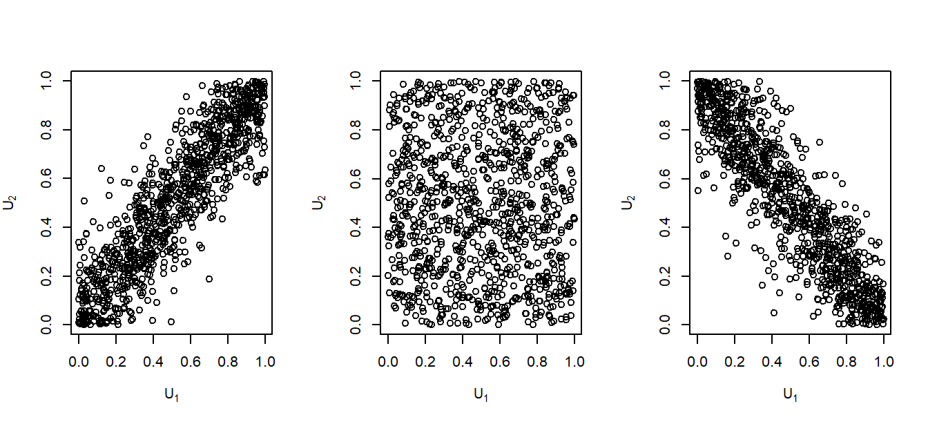
Figure 16.5: Scatterplot of Observations from Frank’s Copula. \(\gamma=12\) (left), \(\gamma=0\) (middle) and \(\gamma=-12\) (right).
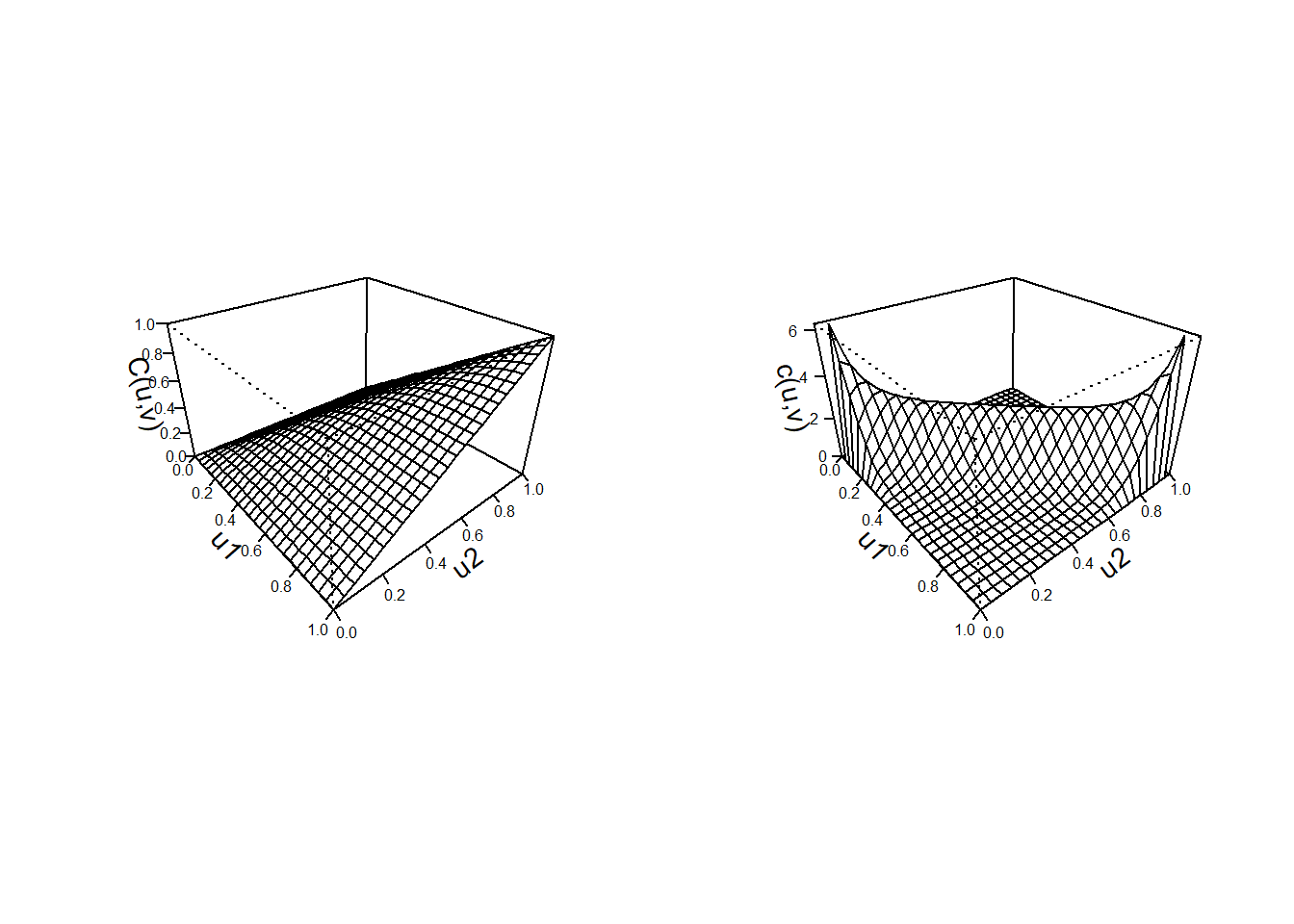
Figure 16.6: Left: Plot for distribution function for Frank’s Copula (\(\gamma=12\)). Right: Plot for the density function for Frank’s Copula (\(\gamma=12\)).
R Code for Frank Copula Plots
Example 16.2.1. Copula Representation Example
Suppose we have a variable \(X\) that follows a Pareto distribution with a scale parameter of \(\theta=10\) and a shape parameter of \(\alpha=1.6\). Additionally, let \(Y\) be an exponential variable with a mean value of 8. Write \(F_{X,Y}(7.2, 4.1)\) in the form \(C(u,v)\).
Note: \(F_{X,Y}(x,y)\) is the joint distribution function and \(C(u,v)\) is the copula that links \(X\) and \(Y\).
Show Example Solution
16.2.2 Sklar’s Theorem
In Sklar (1959), Sklar showcased how copulas can capture the dependence structure of a group of random variables. This principle has since been referred to as Sklar’s Theorem and serves as the cornerstone of copula theory. Dependence modeling with copulas for continuous multivariate distributions allows for the separation of modeling the univariate marginals and the dependence structure, where a copula can represent the dependence structure.
- For a \(p\)-variate distribution \(F\), with marginal cumulative distribution functions \(F_1, \ldots, F_p\), the copula associated with \(F\) is a distribution function \(C: [0,1]^p \rightarrow [0,1]\) with \(U(0,1)\) margins that satisfies:
\[\begin{equation} {F}\left(\mathbf{y}\right)= {C}\left({F}_1\left(y_1\right), \ldots, {F}_p\left(y_p\right)\right), \quad \mathbf{y}=\{y_1 \ldots y_p\} \in \mathbb{R}^p. \tag{16.3} \end{equation}\]
If \(F\) is a continuous \(p\)-variate distribution function with univariate margins \(F_1, \ldots, F_p\) and quantile functions \(F_1^{-1}, \ldots, F_p^{-1}\), then:
\[ C\left(\mathbf{u}\right) =F\left(F_1^{-1}\left(u_1\right), \ldots, F_p^{-1}\left(u_p\right)\right), \quad \mathbf{u} \in [0,1]^p , \]
is the unique choice.
- The converse also holds: If \(C\) is a copula and \(F_1, \ldots, F_p\) are univariate cumulative distribution functions, then the function \(F\) defined by (16.3) is a joint cumulative distribution function with marginal cumulative distribution functions \(F_1, \ldots, F_p\).
Proof of Sklar’s Theorem
According to the first part of Sklar’s theorem, there is a unique underlying copula that is unknown, and it can be estimated from the data available. After estimating the margins and copula, they are usually combined using (16.3) to give the estimated multivariate distribution function. Also, Sklar’s theorem’s second part enables the construction of adaptable multivariate distribution functions with specified univariate margins. These functions are useful in more intricate models, like pricing models.
Show Quiz Solution
16.3 Application Using Copulas
In this section, you learn how to:
- Discover dependence structure between random variables
- Model the dependence with a copula function
This section analyzes the insurance losses and expenses data with the statistical program R. The data set is visualized in Figure 16.1. The model fitting process is started by marginal modeling of each of the two variables, \({\tt LOSS}\) and \({\tt ALAE}\). Then we model the joint distribution of these marginal outcomes.
16.3.1 Marginal Models
We first examine the marginal distributionsThe probability distribution of the variables contained in the subset of a collection of random variables of losses and expenses before going through the joint modeling. The histograms show that both \({\tt LOSS}\) and \({\tt ALAE}\) are right-skewed and fat-tailedA fat-tailed distribution is a probability distribution that exhibits a large skewness or kurtosis, relative to that of either a normal distribution or an exponential distribution. Because of these features, for both marginal distributions of losses and expenses, we consider a Pareto distribution, distribution function of the form
\[ F(y)=1- \left( \frac{\theta}{y+ \theta} \right) ^{\alpha}. \]
Here, \(\theta\) is a scale parameter and \(\alpha\) is a shape parameter. Section 20.2 provides details of this distribution.
The marginal distributions of losses and expenses are fit using the method of maximum likelihood. Specifically, we use the vglm function from the R VGAM package. Firstly, we fit the marginal distribution of \({\tt ALAE}\). Parameters are summarized in Table 16.6.
R Code for Pareto Fitting of ALAE
We repeat this procedure to fit the marginal distribution of the \({\tt LOSS}\) variable. Because the loss variable also seems right-skewed and heavy-tailed data, we also model the marginal distribution with the Pareto distribution (although with different parameters).
R Code for Pareto Fitting of LOSS
Table 16.6. Summary of Pareto Maximum Likelihood Fitted Parameters from the LGPIF Data
\[ {\small \begin{matrix} \begin{array}{l|r|r} \hline & \text{Shape } \hat{\theta} &\text{Scale } \hat{\alpha} \\ \hline ALAE & 15133.60360 & 2.22304 \\ LOSS & 16228.14797 & 1.23766 \\ \hline \end{array} \end{matrix}} \]
To visualize the fitted distribution of \({\tt LOSS}\) and \({\tt ALAE}\) variables, one can use the estimated parameters and plot the corresponding distribution function and density function. For more details on the selection of marginal models, see Chapter 6.
16.3.2 Probability Integral Transformation
When studying simulation, in Section 8.1.2 we learned about the inverse transform methodSamples a uniform number between 0 and 1 to represent the randomly selected percentile, then uses the inverse of the cumulative density function of the desired distribution to simulate from in order to find the simulated value from the desired distribution. This is a way of mapping a \(U(0,1)\) random variable into a random variable \(X\) with distribution function \(F\) via the inverse of the distribution, that is, \(X = F^{-1}(U)\). The probability integral transformationAny continuous variable can be mapped to a uniform random variable via its distribution function goes in the other direction, it states that \(F(X) = U\). Although the inverse transform result is available when the underlying random variable is continuous, discrete or a hybrid combination of the two, the probability integral transform is mainly useful when the distribution is continuous. That is the focus of this chapter.
We use the probability integral transform for two purposes: (1) for diagnostic purposes, to check that we have correctly specified a distribution function and (2) as an input into the copula function in equation (16.1).
For the first purpose, we can check to see whether the Pareto is a reasonable distribution to model our marginal distributions. Given the fitted Pareto distribution, the variable \({\tt ALAE}\) is transformed to the variable \(u_1\), which follows a uniform distribution on \([0,1]\):
\[ u_1 = \hat{F}_{1}(ALAE) = 1 - \left( \frac{\hat{\theta}}{\hat{\theta}+ALAE} \right)^{\hat{\alpha}}. \]
After applying the probability integral transformation to the \({\tt ALAE}\) variable, we plot the histogram of Transformed \({\tt ALAE}\) in Figure 16.7. This plot appears reasonably close to what we expect to see with a uniform distribution, suggesting that the Pareto distribution is a reasonable specification.
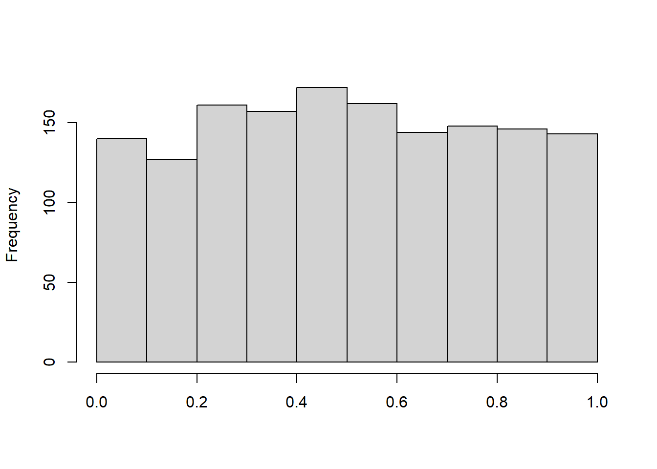
Figure 16.7: Histogram of Transformed ALAE
In the same way, the variable \({\tt LOSS}\) is also transformed to the variable \(u_2\), which follows a uniform distribution on \([0,1]\). The left-hand panel of Figure 16.8 shows a plot the histogram of Transformed \({\tt ALAE}\), again reinforcing the Pareto distribution specification. For another way of looking at the data, the variable \(u_2\) can be transformed to a normal score with the quantile function of standard normal distribution. As we see in Figure 16.8, normal scores of the variable \({\tt LOSS}\) are approximately marginally standard normal. This figure is helpful because analysts are used to looking for patterns of approximate normality (which seems to be evident in the figure). The logic is that, if the Pareto distribution is correctly specified, then transformed losses \(u_2\) should be approximately normal, and the normal scores \(\Phi^{-1}(u_2)\), should be approximately normal. (Here, \(\Phi\) is the cumulative standard normal distribution function.)
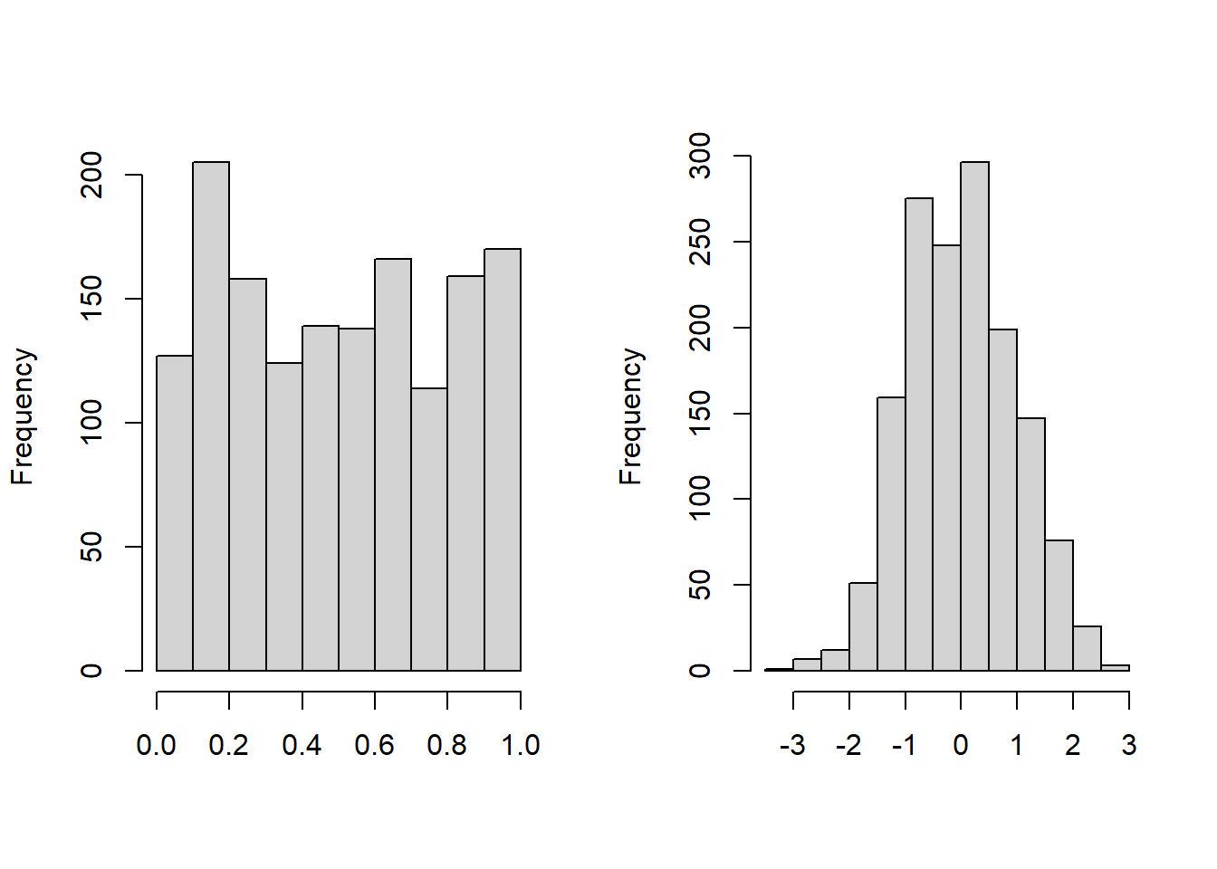
Figure 16.8: Histogram of Transformed Loss. The left-hand panel shows the distribution of probability integral transformed losses. The right-hand panel shows the distribution for the corresponding normal scores.
R Code for Histograms of Transformed Variables
16.3.3 Joint Modeling with Copula Function
Before jointly modeling losses and expenses, we draw the scatterplot of transformed variables \((U_1, U_2)\) and the scatterplot of normal scores in Figure 16.9. The left-hand panel is a plot of \(U_1\) versus \(U_2\), where \(U_1 = \hat{F}_1(ALAE)\) and \(U_2=\hat{F}_2(LOSS)\)). Then we transform each one using an inverse standard normal distribution function, \(\Phi^{-1}(\cdot)\), or qnorm in R to get normal scores. As in Figure 16.1, it is difficult to see patterns in the left-hand panel. However, with rescaling, patterns are evident in the right-hand panel. To learn more details about normal scores and their applications in copula modeling, see Joe (2014).
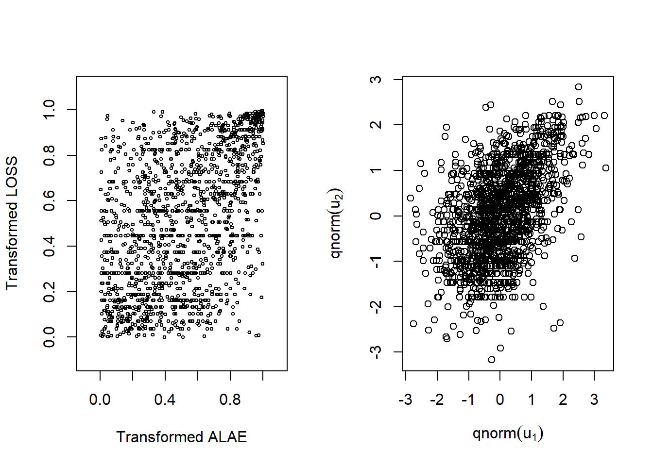
Figure 16.9: Left: Scatter plot for transformed variables. Right:Scatter plot for normal scores
R Code for Scatter Plots and Correlation
The right-hand panel of Figure 16.1 shows us there is a positive dependency between these two random variables. This can be summarized using, for example, Spearman’s rho that turns out to be 0.451. As we learned in Section 16.1.2.1, this statistic depends only on the order of the two variables through their respective ranks. Therefore, the statistic is the same for (1) the original data in Figure 16.1, (2) the data transformed to uniform scales in the left-hand panel of Figure 16.9, and (3) the normal scores in the right-hand panel of Figure 16.9.
The next step is to calculate estimates of the copula parameters. One option is to use traditional maximum likelihood and determine all the parameters at the same time which can be computationally burdensome. Even in our simple example, this means maximizing a (log) likelihood function over five parameters, two for the marginal \({\tt ALAE}\) distribution, two for the marginal \({\tt LOSS}\) distribution, and one for the copula. A widely alternative, known as the inference for margins (IFM) approach, is to simply use the fitted marginal distributions, \(u_1\) and \(u_2\), as inputs when determining the copula. This is the approach taken here. In the following code, you will see that the fitted copula parameter becomes \(\hat{\gamma} = 3.114\).
R Code for IFM Fitting with Frank’s Copula
To visualize the fitted Frank’s copula, the distribution function and density function perspective plots are drawn in Figure 16.10.
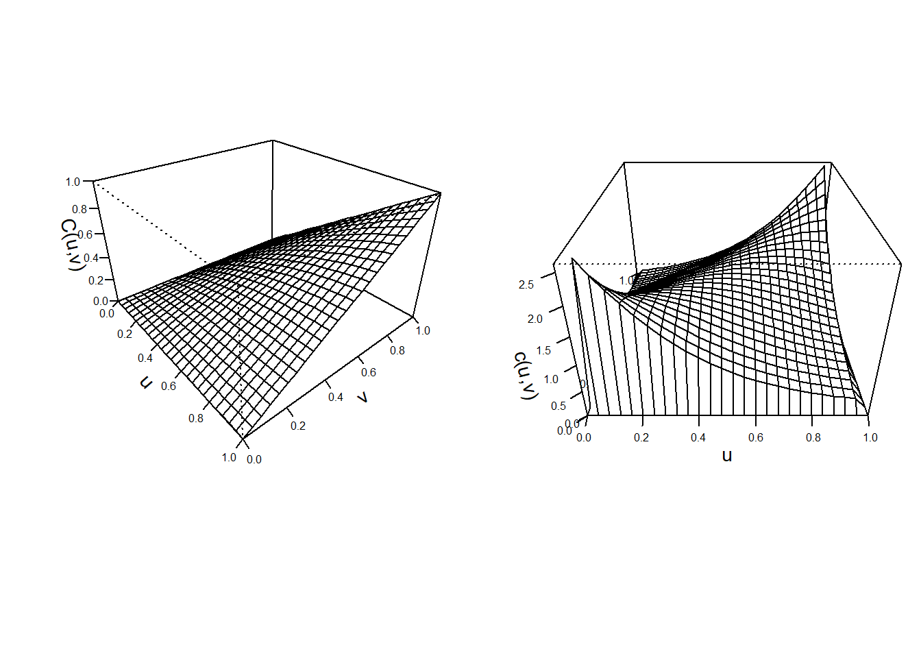
Figure 16.10: Left: Plot for distribution function for Franks Copula. Right:Plot for density function for Franks Copula
R Code for Frank’s Copula Plots
We can estimate the anticipated expenses when losses surpass a specific threshold by utilizing the fitted Frank copula based on the data on losses and expenses. For instance, according to the data, the mean expense when losses exceed \(\$200,000\) is \(\$58,807\). However, when we apply the fitted Frank copula, the projected expenses when losses exceed \(\$200,000\) is \(\$26,767\). This indicates that the Frank copula doesn’t provide an accurate estimate and may not be suitable for this dataset. We will now explore other copula types.
R Code for using the fitted Frank copula to calculate the expected level of expenses
16.4 Types of Copulas
In this section, you learn how to:
- Define the basic types of elliptical copulas, including the normal, \(t\)
- Define basic types of Archimedean copulas
There are several families of copulas that have been described in the literature. Two main families of the copula families are the Archimedean and Elliptical copulas.
16.4.1 Normal (Gaussian) Copulas
We started our study with Frank’s copula in equation (16.2) because it can capture both positive and negative dependence and has a readily understood analytic form. However, extensions to multivariate cases where \(p>2\) are not easy and so we look to alternatives. In particular, the normal, or Gaussian, distribution has been used for many years in empirical work, starting with Gauss in 1887. So, it is natural to turn to this distribution as a benchmark for understanding multivariate dependencies.
For a multivariate normal distribution, think of \(p\) normal random variables, each with mean zero and standard deviation one. Their dependence is controlled by \(\boldsymbol \Sigma\), a correlation matrixA table showing correlation coefficients between variables, with ones on the diagonal. The number in the \(i\)th row and \(j\)th column, say \(\boldsymbol \Sigma_{ij}\), gives the correlation between the \(i\)th and \(j\)th normal random variables. This collection of random variables has a multivariate normal distribution with probability density function
\[\begin{equation} \phi_N (\mathbf{z})= \frac{1}{(2 \pi)^{p/2}\sqrt{\det \boldsymbol \Sigma}} \exp\left( -\frac{1}{2} \mathbf{z}^{\prime} \boldsymbol \Sigma^{-1}\mathbf{z}\right). \tag{16.4} \end{equation}\]
To develop the corresponding copula version, it is possible to start with equation (16.1), evaluate this using normal variables, and go through a bit of calculus. Instead, we simply state as a definition, the normal (Gaussian) copula density function is
\[ c_N(u_1, \ldots, u_p) = \phi_N \left(\Phi^{-1}(u_1), \ldots, \Phi^{-1}(u_p) \right) \prod_{j=1}^p \frac{1}{\phi(\Phi^{-1}(u_j))}. \]
Here, we use \(\Phi\) and \(\phi\) to denote the standard normal distribution and density functions. Unlike the usual probability density function \(\phi_N\), the copula density function has its domain on the hyper-cube \([0,1]^p\). For contrast, Figure 16.11 compares these two density functions.
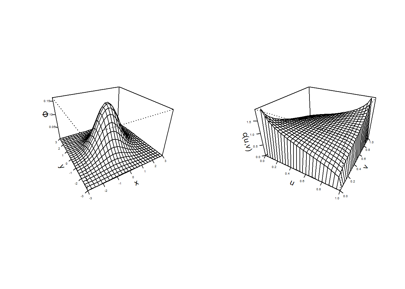
Figure 16.11: Bivariate Normal Probability Density Function Plots. The left-hand panel is a traditional bivariate normal probability density function. The right-hand plot is a plot of the copula density for the normal distribution.
R Code for Normal pdf and Normal Copula pdf Plots
16.4.2 t- and Elliptical Copulas
Another copula used widely in practice is the \(t\)- copula. Both the \(t\)- and the normal copula are special cases of a family known as elliptical copulas, so we introduce this general family first, then specialize to the case of the \(t\)- copula.
The normal and the \(t\)- distributions are examples of symmetric distributions. More generally, elliptical distributionsAny member of a broad family of probability distributions that generalize the multivariate normal distribution is a class of distributions that are symmetric and can be multivariate. In short, an elliptical distribution is a type of symmetric, multivariate distribution. The multivariate normal and multivariate \(t\)- are special types of elliptical distributions.
Elliptical copulasThe copulas of elliptical distributions are constructed from elliptical distributions. This copula decomposes a (multivariate) elliptical distribution into their univariate elliptical marginal distributions by Sklar’s theorem. Properties of elliptical copulas can be obtained from the properties of the corresponding elliptical distributions, see for example, Hofert et al. (2018).
In general, a \(p\)-dimensional vector of random variables has an elliptical distribution if the density can be written as
\[ h_E (\mathbf{z})= \frac{k_p}{\sqrt{\det \boldsymbol \Sigma}} g_p \left( \frac{1}{2} (\mathbf{z}- \boldsymbol \mu)^{\prime} \boldsymbol \Sigma^{-1}(\mathbf{z}- \boldsymbol \mu) \right) , \]
for \(\mathbf{z} \in R^p\) and \(k_p\) is a constant, determined so the density integrates to one. The function \(g_p(\cdot)\) is called a generator because it can be used to produce different distributions. Table 16.7 summarizes a few choices used in actuarial practice. The choice \(g_p(x) = \exp(-x)\) gives rises to the normal pdf in equation (16.4). The choice \(g_p(x) = \exp(-(1+2x/r)^{-(p+r)/2})\) gives rise to a multivariate \(t\)- distribution with \(r\) degrees of freedom with pdf
\[ h_{t_r} (\mathbf{z})= \frac{k_p}{\sqrt{\det \boldsymbol \Sigma}} \exp\left[- \left( 1+ \frac{(\mathbf{z}- \boldsymbol \mu)^{\prime} \boldsymbol \Sigma^{-1}(\mathbf{z}- \boldsymbol \mu)}{r} \right)^{-(p+r)/2}\right] . \]
Table 16.7. Generator Functions (\(g_p(\cdot)\)) for Selected Elliptical Distributions
\[ \small\begin{array}{lc} \hline & Generator \\ Distribution & g_p(x) \\ \hline \text{Normal distribution} & e^{-x}\\ t-\text{distribution with }r \text{ degrees of freedom} & (1+2x/r)^{-(p+r)/2}\\ \text{Cauchy} & (1+2x)^{-(p+1)/2}\\ \text{Logistic} & e^{-x}/(1+e^{-x})^2\\ \text{Exponential power} & \exp(-rx^s)\\ \hline \end{array} \]
We can use elliptical distributions to generate copulas. Because copulas are concerned primarily with relationships, we may restrict our considerations to the case where \(\mu = \mathbf{0}\) and \(\boldsymbol \Sigma\) is a correlation matrix. With these restrictions, the marginal distributions of the multivariate elliptical copula are identical; we use \(H\) to refer to this marginal distribution function and \(h\) is the corresponding density. This marginal density is \(h(z) = k_1 g_1(z^2/2).\) For example, in the normal case we have \(H(\cdot)=\Phi(\cdot)\) and \(h(\cdot)=\phi(\cdot)\).
We are now ready to define the pdf of the elliptical copula, a function defined on the unit cube \([0,1]^p\) as
\[ {c}_E(u_1, \ldots, u_p) = h_E \left(H^{-1}(u_1), \ldots, H^{-1}(u_p) \right) \prod_{j=1}^p \frac{1}{h(H^{-1}(u_j))}. \]
As noted above, most empirical work focuses on the normal copula and \(t\)-copula. Specifically, \(t\)-copulas are useful for modeling the dependency in the tails of bivariate distributions, especially in financial risk analysis applications. The \(t\)-copulas with same association parameter in varying the degrees of freedom parameter show us different tail dependency structures. For more information about \(t\)-copulas, readers can see Joe (2014) and Hofert et al. (2018).
We used the same approach as with the fitted Frank copula to fit the Normal and \(t\) copula. The R code below fits the Normal and \(t\) copula and estimates the expected level of expenses when losses exceed \(\$200,000\). The results show that the estimated expenses using the fitted Normal copula when losses exceed \(\$200,000\) is \(\$35,411\). However, this is not a good fit compared to the mean expense of \(\$58,807\) from the losses and expenses data. When losses exceed \(\$200,000\), the fitted \(t\) copula estimates expenses to be \(\$47,354\), making it a better fit than the Normal copula.
R Code for using the fitted Normal and t copula to calculate the expected level of expenses
16.4.3 Archimedean Copulas
This class of copulas is also constructed from a generator function. For Archimedean copulas, we assume that \(g(\cdot)\) is a convex, decreasing function with domain [0,1] and range \([0, \infty)\) such that \(g(0)=0\). Use \(g^{-1}\) for the inverse function of \(g\). Then the function
\[ C_g(u_1, \ldots, u_p) = g^{-1} \left(g(u_1)+ \cdots + g(u_p) \right) \]
is said to be an Archimedean copula distribution function.
For the bivariate case, \(p=2\), an Archimedean copula function can be written by the function
\[ C_{g}(u_1, \, u_2) = g^{-1} \left(g(u_1) + g(u_2) \right). \]
Some important special cases of Archimedean copulas include the Frank, Clayton/Cook-Johnson, and Gumbel/Hougaard copulas. Each copula class is derived from different generator functions. As another useful special case, recall the Frank’s copula described in Sections 16.2 and 16.3. To illustrate, we now provide explicit expressions for the Clayton and Gumbel/Hougaard copulas.
Clayton Copula
For \(p=2\), the Clayton copula with parameter \(\gamma \in [-1,\infty)\) is defined by
\[ C_{\gamma}^C(u)=\max\{u_1^{-\gamma}+u_2^{-\gamma}-1,0\}^{1/\gamma}, \quad u \in [0,1]^2. \]
This is a bivariate distribution function defined on the unit square \([0,1]^2.\) The range of dependence is controlled by the parameter \(\gamma\), similar to Frank’s copula.
Gumbel-Hougaard Copula
The Gumbel-Hougaard copula is parametrized by \(\gamma \in [1,\infty)\) and defined by
\[ C_{\gamma}^{GH}(u)=\exp\left(-\left(\sum_{i=1}^2 (-\log u_i)^{\gamma}\right)^{1/\gamma}\right), \quad u\in[0,1]^2. \]
For more information on Archimedean copulas, see Joe (2014), Frees and Valdez (1998), and Genest and Mackay (1986).
We used the same approach to fit the Clayton and Gumbel-Hougaard copulas as we did for the fitted Frank copula. The R code below fits these two copulas and determines the expected expense level for losses higher than \(\$200,000\). Our analysis shows that the estimated expenses for losses exceeding \(\$200,000\) using the fitted Clayton copula are \(\$14,209\), while the fitted Gumbel-Hougaard copula predicts \(\$58,554\). Of all the copula types considered, the Gumbel-Hougaard copula provides the best fit for this data. For more on Goodness-of-fit tests, see Hofert et al. (2018).
R Code for using the fitted Clayton and Gumbel-Hougaard copula to calculate the expected level of expenses
Show Quiz Solution
16.5 Properties of Copulas
In this section, you learn how to:
- Interpret bounds that limit copula distribution functions as the amount of dependence varies
- Calculate measures of association for different copulas and interpret their properties
- Interpret tail dependency for different copulas
With many choices of copulas available, it is helpful for analysts to understand general features of how these alternatives behave.
16.5.1 Bounds on Association
Any distribution function is bounded below by zero and from above by one. Additional types of bounds are available in multivariate contexts. These bounds are useful when studying dependencies. That is, as an analyst thinks about variables as being extremely dependent, one has available bounds that cannot be exceeded, regardless of the dependence. The most widely used bounds in dependence modeling are known as the Fréchet-Höeffding bounds, given as
\[ \max( u_1 +\cdots+ u_p - p +1, 0) \leq C(u_1, \ldots, u_p) \leq \min (u_1, \ldots,u_p). \]
To see the right-hand side of this equation, note that
\[ C(u_1,\ldots, u_p) = \Pr(U_1 \leq u_1, \ldots, U_p \leq u_p) \leq \Pr(U_j \leq u_j), \]
for \(j=1,\ldots,p\). The bound is achieved when \(U_1 = \cdots = U_p\). To see the left-hand side when \(p=2\), consider \(U_2=1-U_1\). In this case, if \(1-u_2 < u_1\) then
\[ \Pr(U_1 \leq u_1, U_2 \leq u_2) = \Pr ( 1-u_2 \leq U_1 < u_1) =u_1+u_2-1. \] See, for example, Nelson (1997) for additional discussion.
To see how these bounds relate to the concept of dependence, consider the case of \(p=2\). As a benchmark, first note that the product copula, \(C(u_1,u_2)=u_1 \cdot u_2\), is the result of assuming independence between random variables. Now, from the above discussion, we see that the lower bound is achieved when the two random variables are perfectly negatively related (\(U_2=1-U_1\)). Further, it is clear that the upper bound is achieved when they are perfectly positively related (\(U_2=U_1\)). To emphasize this, the Frechet-Hoeffding boundsBounds of multivariate distribution functions for two random variables appear in Figure 16.12.
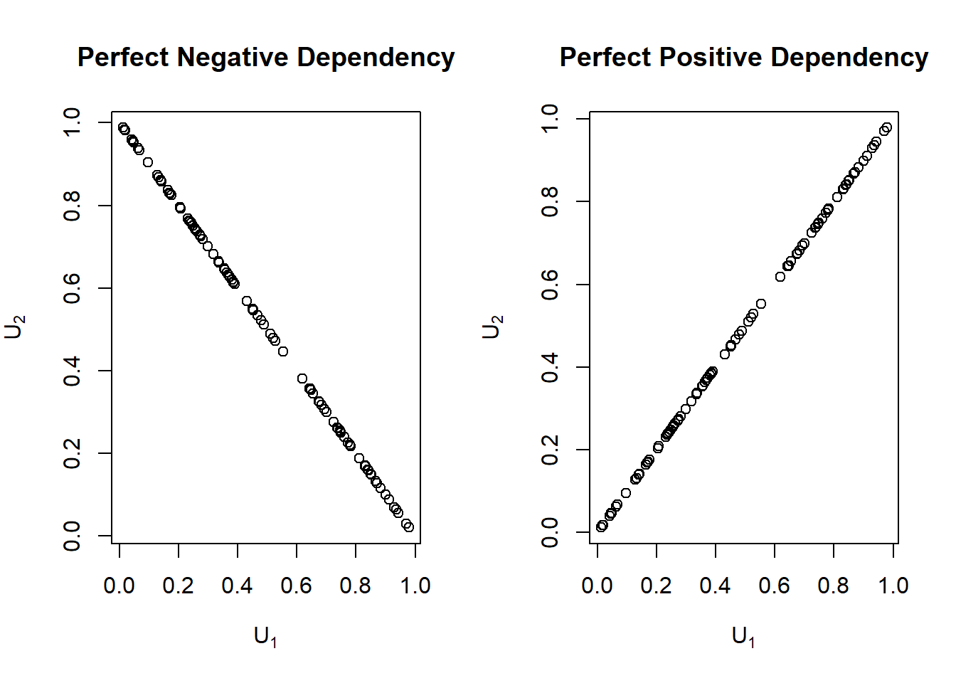
Figure 16.12: Perfect Positive and Perfect Negative Dependence Plots
R Code for the Fréchet-Höeffding Bounds for Two Random Variables
Let’s assign the Fréchet-Höeffding lower bound as \(W\) and the upper bound as \(M\). That is, \(W=\max(u_1+\cdots+u_p-p+1, 0)\) and \(M=\min(u_1,\ldots,u_p)\). It’s important to note that \(W\) is a copula only if \(p=2\), while \(M\) is a copula for all \(p\geq2\). In dimension two, \(W=\max(u_1+u_2-1, 0)\) is known as the counter-monotone copula. It captures the inverse relationship between two variables, that is, two random variables that are perfectly negatively related. On the other hand, \(M=\min(u_1,u_2)\) in dimension two is known as the co-monotone copula. It captures the relationship between two variables where one is related to the other by a strictly increasing function, that is, two random variables that are perfectly positively dependent. The co-monotonic copulas can be extended to the multivariate case. However, it’s not possible to extend the counter-monotonic copula because it’s not possible to have three or more variables where each pair has a direct inverse relationship.
Example 16.5.1. Largest Possible Value Example
Suppose we have a variable \(X\) that follows a Pareto distribution with a scale parameter of \(\theta=10\) and a shape parameter of \(\alpha=1.6\). Additionally, let \(Y\) be an exponential variable with a mean value of 8. Let \(F_{X,Y}(x,y)\) be the joint distribution function. What is the largest possible value of \(F_{X,Y}(7.2,4.1)\)?
Show Example Solution
16.5.2 Measures of Association
Empirical versions of Spearman’s rho and Kendall’s tau were introduced in Sections 16.1.2.1 and 16.1.2.2, respectively. The interesting thing about these expressions is that these summary measures of association are based only on the ranks of each variable. Thus, any strictly increasing transform does not affect these measures of association. Specifically, consider two random variables, \(Y_1\) and \(Y_2\), and let m\(_1\) and m\(_2\) be strictly increasing functions. Then, the association, when measured by Spearman’s rho or Kendall’s tau, between \(m_1(Y_1)\) and \(m_2(Y_2)\) does not change regardless of the choice of m\(_1\) and m\(_2\). For example, this allows analysts to consider dollars, Euros, or log dollars, and still retain the same essential dependence. As we have seen in Section 16.1, this is not the case with the Pearson’s measure of correlation.
Schweizer, Wolff, and others (1981) established that the copula accounts for all the dependence in the sense that the way \(Y_1\) and \(Y_2\) “move together” is captured by the copula, regardless of the scale in which each variable is measured. They also showed that (population versions of) the two standard nonparametric measures of association could be expressed solely in terms of the copula function. Spearman’s correlation coefficient is given by
\[\begin{equation} \rho_S = 12 \int_0^1 \int_0^1 \left\{C(u,v) - uv \right\} du dv. \tag{16.5} \end{equation}\]
Kendall’s tau is given by
\[ \tau= 4 \int_0^1 \int_0^1 C(u,v)~dC(u,v) - 1 . \]
For these expressions, we assume that \(Y_1\) and \(Y_2\) have a jointly continuous distribution function.
Example. Loss versus Expenses. Earlier, in Section 16.3, we saw that the Spearman’s correlation was 0.452, calculated with the rho function. Then, we fit Frank’s copula to these data, and estimated the dependence parameter to be \(\hat{\gamma} = 3.114\). As an alternative, the following code shows how to use the empirical version of equation (16.5). In this case, the Spearman’s correlation coefficient is 0.462, which is close to the sample Spearman’s correlation coefficient, 0.452.
R Code for Spearman’s Correlation Using Frank’s Copula
16.5.3 Tail Dependency
As discussed in Section 16.1.3, there are applications in which it is useful to distinguish the part of the distribution in which the association is strongest. For example, in insurance it is helpful to understand association among the largest losses, that is, association in the right tails of the data. This subsection defines upper and lower tail dependency in terms of copulas.
To capture this type of dependency, we use the right-tail concentration function, defined as
\[ R(z) = \frac{\Pr(U_1 >z, U_2 > z)}{1-z} =\Pr(U_1 > z | U_2 > z) =\frac{1 - 2z + C(z,z)}{1-z} . \]
As a benchmark, \(R(z)\) will be equal to \(z\) under independence. Joe (1997) uses the term “upper tail dependence parameter” for \(R = \lim_{z \rightarrow 1} R(z)\).
In the same way, one can define the left-tail concentration function as
\[ L(z) = \frac{\Pr(U_1 \leq z, U_2 \leq z)}{z}=\Pr(U_1 \leq z | U_2 \leq z) =\frac{ C(z,z)}{z}, \]
with the lower tail dependence parameter \(L = \lim_{z \rightarrow 0} L(z)\). A tail dependencyA measure of their comovements in the tails of the distributions concentration function captures the probability of two random variables simultaneously having extreme values.
It is of interest to see how well a given copula can capture tail dependence. To this end, we calculate the left and right tail concentration functions for four different types of copulas; Normal, Frank, Gumbel and \(t\)- copulas. The results are summarized for concentration function values for these four copulas in Table 16.8. As in Gary G. Venter (2002), we show \(L(z)\) for \(z\leq 0.5\) and \(R(z)\) for \(z>0.5\) in the tail dependence plot in Figure 16.13. We interpret the tail dependence plot to mean that both the Frank and Normal copula exhibit no tail dependence whereas the \(t\)- and the Gumbel do so. The \(t\)- copula is symmetric in its treatment of upper and lower tails.
Table 16.8. Tail Dependence Parameters for Four Copulas
\[ {\small \begin{matrix} \begin{array}{l|rr} \hline \text{Copula} & \text{Lower} & \text{Upper} \\ \hline \text{Frank} & 0 & 0 \\ \text{Gumbel} & 0 & 0.74 \\ \text{Normal} & 0 & 0 \\ t- & 0.10 & 0.10 \\ \hline \end{array} \end{matrix}} \]
R Code for Tail Copula Functions for Different Copulas
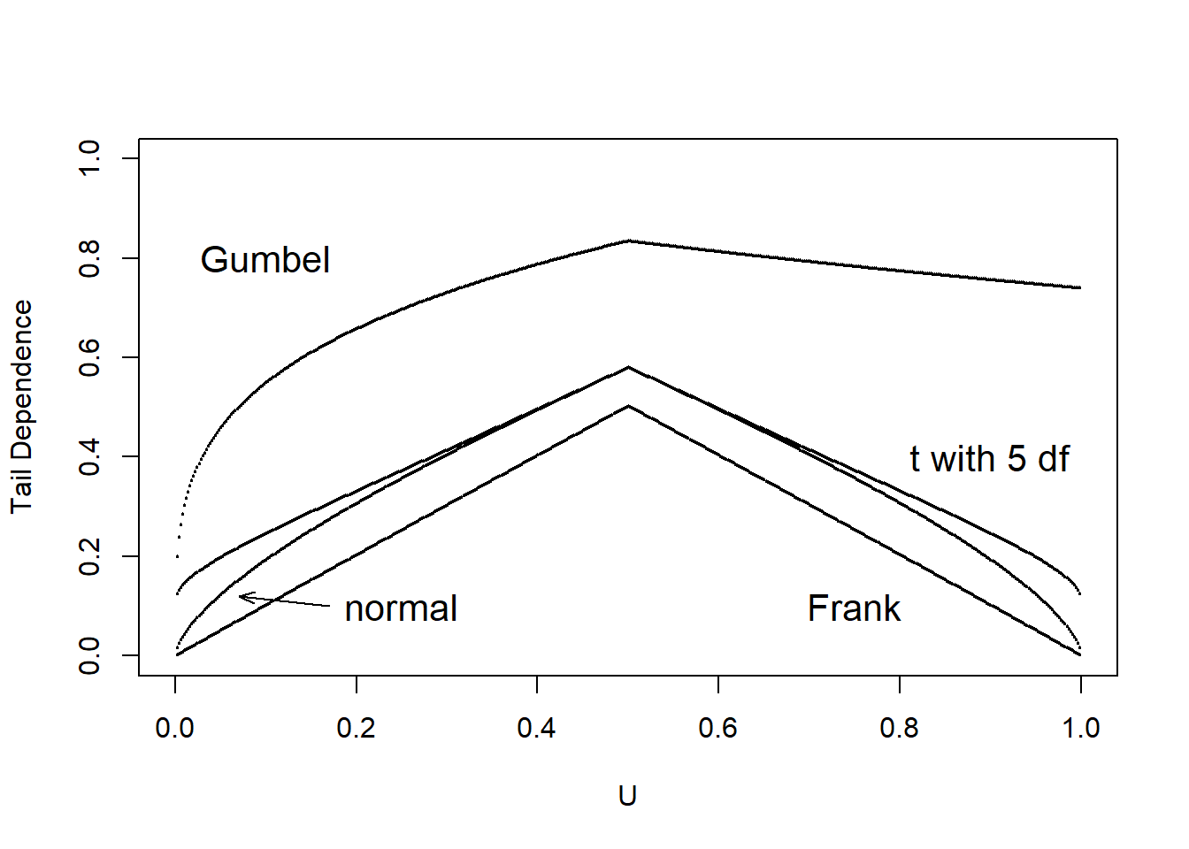
Figure 16.13: Tail Dependence Plots
R Code for Tail Dependence Plot for Different Copulas
Example 16.5.2. Lower Tail Dependence Coefficient Example
The bivariate distribution function \(C(u,v)=uv\). What is the lower tail dependence coefficient of this copula?
Show Example Solution
Show Quiz Solution
16.6 Importance of Dependence Modeling
In this section, you learn how to:
- Explain the importance of dependence modeling
- Explain the importance of copulas for regression applications
16.6.1 Why is Dependence Modeling Important?
Dependence modeling is important because it enables us to understand the dependence structure by defining the relationship between variables in a dataset. In insurance, ignoring dependence modeling may not impact pricing but could lead to misestimation of required capital to cover losses. For instance, from Section 16.3 , it is seen that there was a positive relationship between \({\tt LOSS}\) and \({\tt ALAE}\). This means that, if there is a large loss then we expect expenses to be large as well and ignoring this relationship could lead to mis-estimation of reserves.
To illustrate the importance of dependence modeling, we refer you back to portfolio management example in Section 13.4.3.3 that assumed that the property and liability risks are independent. Now, we incorporate dependence by allowing the four lines of business to depend on one another through a Gaussian copula. In Table 16.9, we show that dependence affects the portfolio quantiles (\(VaR_q\)), although not the expected values. For instance, the \(VaR_{0.99}\) for total risk which is the amount of capital required to ensure, with a \(99\%\) degree of certainty that the firm does not become technically insolvent is higher when we incorporate dependence. This leads to less capital being allocated when dependence is ignored and can cause unexpected solvency problems.
Table 16.9. Results for Portfolio Expected Value and Quantiles (\(VaR_q\))
\[ {\small \begin{matrix} \begin{array}{l|rrrr} \hline \text{Independent} &\text{Expected} & VaR_{0.9} & VaR_{0.95} & VaR_{0.99} \\ &\text{Value} & & & \\ \hline \text{Retained} & 269 & 300 & 300 & 300 \\ \text{Insurer} & 2,274 & 4,400 & 6,173 & 11,859 \\ \text{Total} & 2,543 & 4,675 & 6,464 & 12,159 \\ \hline \text{Gaussian Copula}&\text{Expected}& VaR_{0.9} & VaR_{0.95} & VaR_{0.99} \\ &\text{Value} & & & \\ \hline \text{Retained} & 269 & 300 & 300 & 300 \\ \text{Insurer} & 2,340 & 4,988 & 7,339 & 14,905 \\ \text{Total} & 2,609 & 5,288 & 7,639 & 15,205 \\ \hline \end{array} \end{matrix}} \]
R Code for Simulation Using Gaussian Copula
It should be noted that there are various methods of conducting dependence modeling, but copulas are effective for many actuarial applications. It’s important to stress that each copula function captures a distinct dependency structure based on its functional form and dependence parameters. Therefore, utilizing copulas without comprehending their limitations and properties can lead to biased and statistically incorrect results. Since selecting the right copula involves extensive effort, here are some general tips that can assist:
When analyzing data, diagnostic and exploratory analysis can provide insight into the dependence structure of the data, which can help determine suitable copula functions. For Archimedean Copulas specifically, understanding the dependence structure can narrow down the appropriate type of copula function. For instance, the Gumbel-Hougaard copula is not suitable for negative dependency, but the Frank Copula can effectively capture three distinct types of dependency in the data.
Researchers cannot rely on Normal copula or Frank copula functions to capture the upper and lower tail dependency in data. Instead, a \(t\) copula with low degrees of freedom works well for both tails. The Gumbel-Hougaard copula shows some upper tail dependence but less or no lower tail dependence, while the Clayton copula exhibits strong lower tail dependence.
16.6.2 Copula Regression
In regression studies, the response variable is determined by a group of explanatory variables. This is often one of the initial statistical methods used to understand the connection between the response and explanatory variables. However, Linear Models and Generalized Linear Models can impose constraints on the selection of distributions for the response variables, which can be restrictive for practical data scenarios. For example, insurance claim amounts and financial asset returns typically exhibit heavy-tailed and skewed distributions, and may not adhere to normality patterns, with the possibility of having extreme values.
The use of copulas in regression is gaining attention in the field of actuarial science. Copula regression separates the dependency structure from the selection of marginal distributions, allowing for greater flexibility in choosing distributions for actuarial applications. The parameters for the marginal distributions and the copula distribution can be estimated either separately or together. The maximum likelihood method is often effective for estimating the parameters. However, for copula regression parameter estimation, the inference for margins method (IFM) is commonly used. Copula functions preserve the marginals and make predictions using the dependent variable’s conditional mean given the covariates. See Krämer et al. (2013), Parsa and Klugman (2011); for detailed examples on copula regression.
Show Quiz Solution
16.7 Further Resources and Contributors
Contributors
- Edward W. (Jed) Frees and Nii-Armah Okine, University of Wisconsin-Madison, and Emine Selin Sarıdaş, Mimar Sinan University, are the principal authors of the initial version of this chapter.
- Chapter reviewers include: Runhuan Feng, Fei Huang, Himchan Jeong, Min Ji, and Toby White.
- Nii-Armah Okine, Appalachian State University, and Emine Selin Sarıdaş, Mimar Sinan University, are the principal authors of the second edition of this chapter. Email: okinean@appstate.edu and selin.saridas@msgsu.edu.tr for chapter comments and suggested improvements.
TS 16.A. Other Classic Measures of Scalar Associations
TS 16.A.1. Blomqvist’s Beta
Blomqvist (1950) developed a measure of dependence now known as Blomqvist’s beta, also called the median concordance coefficient and the medial correlation coefficient. Using distribution functions, this parameter can be expressed as
\[\begin{equation*} \beta_B = 4F\left(F^{-1}_X(1/2),F^{-1}_Y(1/2) \right) - 1. \end{equation*}\]
That is, first evaluate each marginal at its median (\(F^{-1}_X(1/2)\) and \(F^{-1}_Y(1/2)\), respectively). Then, evaluate the bivariate distribution function at the two medians. After rescaling (multiplying by 4 and subtracting 1), the coefficient turns out to have a range of \([-1,1]\), where 0 occurs under independence.
Like Spearman’s rho and Kendall’s tau, an estimator based on ranks is easy to provide. First write \(\beta_B = 4C(1/2,1/2)-1 = 2\Pr((U_1-1/2)(U_2-1/2))-1\) where \(U_1, U_2\) are uniform random variables. Then, define
\[ \hat{\beta}_B = \frac{2}{n} \sum_{i=1}^n I\left( (R(X_{i})-\frac{n+1}{2})(R(Y_{i})-\frac{n+1}{2}) \ge 0 \right)-1 . \]
See, for example, Joe (2014), page 57 or Hougaard (2000), page 135, for more details.
Because Blomqvist’s parameter is based on the center of the distribution, it is particularly useful when data are censored; in this case, information in extreme parts of the distribution are not always reliable. How does this affect a choice of association measures? First, recall that association measures are based on a bivariate distribution function. So, if one has knowledge of a good approximation of the distribution function, then calculation of an association measure is straightforward in principle. Second, for censored data, bivariate extensions of the univariate Kaplan-Meier distribution function estimator are available. For example, the version introduced in Dabrowska (1988) is appealing. However, because of instances when large masses of data appear at the upper range of the data, this and other estimators of the bivariate distribution function are unreliable. This means that, summary measures of the estimated distribution function based on Spearman’s rho or Kendall’s tau can be unreliable. For this situation, Blomqvist’s beta appears to be a better choice as it focuses on the center of the distribution. Hougaard (2000), Chapter 14, provides additional discussion.
You can obtain the Blomqvist’s beta, using the betan() function from the copula library in R. From below, \(\beta_B=0.3\) between the \({\tt Coverage}\) rating variable in millions of dollars and \({\tt Claim}\) amount variable in dollars.
R Code for Blomqvist’s Beta
In addition, to show that the Blomqvist’s beta is invariant under strictly increasing transformations, \(\beta_B=0.3\) between the \({\tt Coverage}\) rating variable in logarithmic millions of dollars and \({\tt Claim}\) amount variable in dollars.
TS 16.A.2. Nonparametric Approach Using Spearman Correlation with Tied Ranks
For the first variable, the average rank of observations in the \(s\)th row is
\[\begin{equation*} r_{1s} = n_{m_1\bullet}+ \cdots+ n_{s-1,\bullet}+ \frac{1}{2} \left(1+ n_{s\bullet}\right) \end{equation*}\]
and similarly \(r_{2t} = \frac{1}{2} \left[(n_{\bullet m_1}+ \cdots+ n_{\bullet,s-1}+1)+ (n_{\bullet m_1}+ \cdots+ n_{\bullet s})\right]\). With this, we have Spearman’s rho with tied rank is
\[\begin{equation*} \hat{\rho}_S = \frac{\sum_{s=m_1}^{m_2} \sum_{t=m_1}^{m_2} n_{st}(r_{1s} - \bar{r})(r_{2t} - \bar{r})} {\left[\sum_{s=m_1}^{m_2}n_{s \bullet}(r_{1s} - \bar{r})^2 \sum_{t=m_1}^{m_2} n_{\bullet t}(r_{2t} - \bar{r})^2 \right]^2} \end{equation*}\]
where the average rank is \(\bar{r} = (n+1)/2\).
Click to Show Proof for Special Case: Binary Data.
You can obtain the ties-corrected Spearman correlation statistic \(r_S\) using the cor() function in R and selecting the spearman method. From below \(\hat{\rho}_S=-0.09\).