Chapter 4 Modeling Loss Severity

Chapter Preview. The traditional loss distribution approach to modeling aggregate lossesAggregate claims, or total claims observed in the time period starts by separately fitting a frequency distribution to the number of losses and a severity distribution to the size of losses. The estimated aggregate loss distribution combines the loss frequency distribution and the loss severity distribution by convolution. Discrete distributions often referred to as counting or frequency distributions were used in Chapter 3 to describe the number of events such as number of accidents to the driver or number of claims to the insurer. Lifetimes, asset values, losses and claim sizes are usually modeled as continuous random variables and as such are modeled using continuous distributions, often referred to as loss or severity distributions. A mixture distributionA weighted average of other distributions, which may be continuous or discrete is a weighted combination of simpler distributions that is used to model phenomenon investigated in a heterogeneous population, such as modeling more than one type of claims in liability insuranceInsurance that compensates an insured for loss due to legal liability towards others (small frequent claims and large relatively rare claims). In this chapter we explore the use of continuous as well as mixture distributions to model the random size of loss.

Sections 4.1 to 4.3 present key attributes that characterize continuous models and means of creating new distributions from existing ones. Section 4.4.1 describes some principal non-parametric methods for estimating loss distributions: moment and percentile based, empirical, and density estimation methods. Section 4.4.2 covers parametric estimation methods including method of moments and percentile matching, and deepens our understanding of maximum likelihood methods. The frequency distributions from Chapter 3 will be combined with the ideas from this chapter to describe the aggregate losses over the whole portfolio in Chapter 7.

4.1 Basic Distributional Quantities

---

In this section, you learn how to define some basic distributional quantities:

• moments,
• moment generating functions, and
• percentiles

---

4.1.1 Moments and Moment Generating Functions

Let \(X\) be a continuous random variableRandom variable which can take infinitely many values in its specified domain with probability density function (pdf) \(f_{X}\left( x \right)\) and distribution function \(F_{X}\left( x \right)\). The k-th raw momentThe kth moment of a random variable x is the average (expected) value of x^k of \(X\), denoted by \(\mu_{k}^{\prime}\), is the expected valueAverage of the k-th power of \(X\), provided it exists. The first raw moment \(\mu_{1}^{\prime}\) is the mean of \(X\) usually denoted by \(\mu\). The formula for \(\mu_{k}^{\prime}\) is given as

\[ \mu_{k}^{\prime} = \mathrm{E}\left( X^{k} \right) = \int_{0}^{\infty}{x^{k}f_{X}\left( x \right)dx } . \] The support of the random variable \(X\) is assumed to be nonnegative since actuarial phenomena are rarely negative. For example, an easy integration by parts shows that the raw moments for nonnegative variables can also be computed using

\[ \mu_{k}^{\prime} = \int_{0}^{\infty}{k~x^{k-1}\left[1- F_{X}(x) \right]dx }, \] that is based on the survival function, denoted as \(S_X(x) = 1-F_{X}(x)\). This formula is particularly useful when \(k=1\). Section 5.1.2 discusses this approach in more detail.

The k-th central momentThe kth central moment of a random variable x is the expected value of (x-its mean)^k of \(X\), denoted by \(\mu_{k}\), is the expected value of the k-th power of the deviation of \(X\) from its mean \(\mu\). The formula for \(\mu_{k}\) is given as

\[ \mu_{k} = \mathrm{E}\left\lbrack {(X - \mu)}^{k} \right\rbrack = \int_{0}^{\infty}{\left( x - \mu \right)^{k}f_{X}\left( x \right) dx }. \] The second central moment \(\mu_{2}\) defines the varianceSecond central moment of a random variable x, measuring the expected squared deviation of between the variable and its mean of \(X\), denoted by \(\sigma^{2}\). The square root of the variance is the standard deviationThe square-root of variance \(\sigma\).

From a classical perspective, further characterization of the shape of the distribution includes its degree of symmetry as well as its flatness compared to the normal distribution. The ratio of the third central moment to the cube of the standard deviation \(\left( \mu_{3} / \sigma^{3} \right)\) defines the coefficient of skewnessMeasure of the symmetry of a distribution, 3rd central moment/standard deviation^3 which is a measure of symmetry. A positive coefficient of skewness indicates that the distribution is skewed to the right (positively skewed). The ratio of the fourth central moment to the fourth power of the standard deviation \(\left(\mu_{4} / \sigma^{4} \right)\) defines the coefficient of kurtosisMeasure of the peaked-ness of a distribution, 4th central moment/standard deviation^4. The normal distribution has a coefficient of kurtosis of 3. Distributions with a coefficient of kurtosis greater than 3 have heavier tails than the normal, whereas distributions with a coefficient of kurtosis less than 3 have lighter tails and are flatter. Section 13.2 describes the tails of distributions from an insurance and actuarial perspective.

Example 4.1.1. Actuarial Exam Question. Assume that the rvRandom variable \(X\) has a gamma distribution with mean 8 and skewness 1. Find the variance of \(X\). (Hint: The gamma distribution is reviewed in Section 4.2.1.)

Show Example Solution

Solution. The pdf of \(X\) is given by

\[ f_{X}\left( x \right) = \frac{\left( x / \theta \right)^{\alpha}}{x ~\Gamma\left( \alpha \right)} e^{- x / \theta} \] for \(x > 0\). For \(\alpha>0\), the k-th raw moment is

\[ \mu_{k}^{\prime} = \mathrm{E}\left( X^{k} \right) = \int_{0}^{\infty}{\frac{1}{\Gamma\left( \alpha \right)\theta^{\alpha}}x^{k + \alpha - 1}e^{- x / \theta} dx} = \frac{\Gamma\left( k + \alpha \right)}{\Gamma\left( \alpha \right)}\theta^{k} \] Given \(\Gamma\left( r + 1 \right) = r\Gamma\left( r \right)\) and \(\Gamma\left( 1 \right) = 1\), then \(\mu_{1}^{\prime} = \mathrm{E}\left( X \right) = \alpha\theta\), \(\mu_{2}^{\prime} = \mathrm{E}\left( X^{2} \right) = \left( \alpha + 1 \right)\alpha\theta^{2}\), \(\mu_{3}^{\prime} = \mathrm{E}\left( X^{3} \right) = \left( \alpha + 2 \right)\left( \alpha + 1 \right)\alpha\theta^{3}\), and \(\mathrm{Var}\left( X \right) = (\alpha + 1)\alpha\theta^2 - (\alpha\theta)^2 = \alpha\theta^{2}\).

\[ \begin{array}{ll} \text{Skewness} &= \frac{\mathrm{E}\left\lbrack {(X - \mu_{1}^{\prime})}^{3} \right\rbrack}{{\left( \mathrm{Var}X \right)}^{3/2}} = \frac{\mu_{3}^{\prime} - 3\mu_{2}^{\prime}\mu_{1}^{\prime} + 2{\mu_{1}^{\prime}}^{3}}{{\left(\mathrm{Var} X \right)}^{3/2}} \\ &= \frac{\left( \alpha + 2 \right)\left( \alpha + 1 \right)\alpha\theta^{3} - 3\left( \alpha + 1 \right)\alpha^{2}\theta^{3} + 2\alpha^{3}\theta^{3}}{\left( \alpha\theta^{2} \right)^{3/2}} \\ &= \frac{2}{\alpha^{1/2}} = 1. \end{array} \]

Hence, \(\alpha = 4\). Since, \(\mathrm{E}\left( X \right) = \alpha\theta = 8\), then \(\theta = 2\) and finally, \(\mathrm{Var}\left( X \right) = \alpha\theta^{2} = 16\).

---

The moment generating function (mgf)The mgf of random variable n is defined the expectation of exp(tn), as a function of t, denoted by \(M_{X}(t)\) uniquely characterizes the distribution of \(X\). While it is possible for two different distributions to have the same moments and yet still differ, this is not the case with the moment generating function. That is, if two random variables have the same moment generating function, then they have the same distribution. The moment generating function is given by \[ M_{X}(t) = \mathrm{E}\left( e^{tX} \right) = \int_{0}^{\infty}{e^{\text{tx}}f_{X}\left( x \right) dx } \] for all \(t\) for which the expected value exists. The mgf is a real function whose k-th derivative at zero is equal to the k-th raw moment of \(X\). In symbols, this is \[ \left.\frac{d^k}{dt^k} M_{X}(t)\right|_{t=0} = \mathrm{E}\left( X^{k} \right) . \]

Example 4.1.2. Actuarial Exam Question. The random variable \(X\) has an exponential distribution with mean \(\frac{1}{b}\). It is found that \(M_{X}\left( - b^{2} \right) = 0.2\). Find \(b\). (Hint: The exponential is a special case of the gamma distribution which is reviewed in Section 4.2.1.)

Show Example Solution

Solution.

With \(X\) having an exponential distribution with mean \(\frac{1}{b}\), we have that \[ M_{X}(t) = \mathrm{E}\left( e^{tX} \right) = \int_{0}^{\infty}{e^{\text{tx}}be^{- bx} dx} = \int_{0}^{\infty}{be^{- x\left( b - t \right)} dx} = \frac{b}{\left( b - t \right)}. \]

Then, \[ M_{X}\left( - b^{2} \right) = \frac{b}{\left( b + b^{2} \right)} = \frac{1}{\left( 1 + b \right)} = 0.2. \] Thus, \(b = 4\).

---

Example 4.1.3. Actuarial Exam Question. Let \(X_{1}, \ldots, X_{n}\) be independentTwo variables are independent if conditional information given about one variable provides no information regarding the other variable random variables, where \(X_i\) has a gamma distribution with parameters \(\alpha_{i}\) and \(\theta\). Find the distribution of \(S = \sum_{i = 1}^{n}X_{i}\), the mean \(\mathrm{E}(S)\), and the variance \(\mathrm{Var}(S)\).

Show Example Solution

Solution.

The mgf of \(S\) is \[ M_{S}(t) = \text{E}\left( e^{\text{tS}} \right) = \mathrm{E}\left( e^{t\sum_{i = 1}^{n}X_{i}} \right) = \mathrm{E}\left( \prod_{i = 1}^{n}e^{tX_{i}} \right) . \] Using independence, we get
\[ M_{S}(t) = \prod_{i = 1}^{n}{\mathrm{E}\left( e^{tX_{i}} \right) = \prod_{i = 1}^{n}{M_{X_{i}}(t)}} . \]

The moment generating function of the gamma distribution \(X_i\) is \(M_{X_i}(t) = (1-\theta t)^{\alpha_i}\). Then, \[ M_{S}(t) = \prod_{i = 1}^{n}\left( 1 - \theta t \right)^{- \alpha_{i}} = \left( 1 - \theta t \right)^{- \sum_{i = 1}^{n}\alpha_{i}} . \] This indicates that the distribution of \(S\) is gamma with parameters \(\sum_{i = 1}^{n}\alpha_{i}\) and \(\theta\).

This is a demonstration of how we can use the uniqueness property of the moment generating function to determine the probability distribution of a function of random variables.

We can find the mean and variance from the properties of the gamma distribution. Alternatively, by finding the first and second derivatives of \(M_{S}(t)\) at zero, we can show that \(\mathrm{E}\left( S \right) = \left. \ \frac{\partial M_{S}(t)}{\partial t} \right|_{t = 0} = \alpha\theta\) where \(\alpha = \sum_{i = 1}^{n}\alpha_{i}\), and

\[ \mathrm{E}\left( S^{2} \right) = \left. \ \frac{\partial^{2}M_{S}(t)}{\partial t^{2}} \right|_{t = 0} = \left( \alpha + 1 \right)\alpha\theta^{2}. \] Hence, \(\mathrm{Var}\left( S \right) = \alpha\theta^{2}\).

---

One can also use the moment generating function to compute the probability generating function

\[ P_{X}(z) = \mathrm{E}\left( z^{X} \right) = M_{X}\left( \log z \right) . \]

As introduced in Section 3.2.2, the probability generating function is more useful for discrete random variables.

---

4.1.2 Quantiles

Quantiles can also be used to describe the characteristics of the distribution of \(X\). When the distribution of \(X\) is continuous, for a given fraction \(0 \leq p \leq 1\) the corresponding quantile is the solution of the equation \[ F_{X}\left( \pi_{p} \right) = p . \] For example, the middle point of the distribution, \(\pi_{0.5}\), is the median50th percentile of a definition, or middle value where half of the distribution lies below. A percentileThe pth percentile of a random variable x is the smallest value x_p such that the probability of not exceeding it is p% is a type of quantile; a \(100p\) percentile is the number such that \(100 \times p\) percent of the data is below it.

Example 4.1.4. Actuarial Exam Question. Let \(X\) be a continuous random variable with density function \(f_{X}\left( x \right) = \theta e^{- \theta x}\), for \(x > 0\) and 0 elsewhere. If the median of this distribution is \(\frac{1}{3}\), find \(\theta\).

Show Example Solution

Solution.

The distribution function is \(F_{X}\left( x \right) = 1 - e^{- \theta x}\). So, \(F_{X}\left( \pi_{0.5} \right) = 1 - e^{- \theta\pi_{0.5}} = 0.5\). As, \(\pi_{0.5} = \frac{1}{3}\), we have \(F_X\left(\frac{1}{3}\right) = 1 - e^{-\theta / 3} = 0.5\) and \(\theta = 3 \log 2\).

---

Section 4.4.1.3 extends the definition of quantiles to include distributions that are discrete, continuous, or a hybrid combination.

Show Quiz Solution

---

---

4.2 Continuous Distributions for Modeling Loss Severity

---

In this section, you learn how to define and apply four fundamental severity distributions:

• gamma,
• Pareto,
• Weibull, and
• generalized beta distribution of the second kind.

---

4.2.1 Gamma Distribution

Recall that the traditional approach in modeling losses is to fit separate models for frequency and claim severity. When frequency and severity are modeled separately it is common for actuaries to use the Poisson distribution (introduced in Section 3.2.3.2) for claim count and the gamma distribution to model severity. An alternative approach for modeling losses that has recently gained popularity is to create a single model for pure premium (average claim cost) that will be described in Chapter 6.

The continuous variable \(X\) is said to have the gamma distribution with shape parameter \(\alpha\) and scale parameter \(\theta\) if its probability density function is given by \[ f_{X}\left( x \right) = \frac{\left( x/ \theta \right)^{\alpha}}{x~ \Gamma\left( \alpha \right)}\exp \left( -x/ \theta \right) \ \ \ \text{for } x > 0 . \] Note that \(\alpha > 0,\ \theta > 0\).

The two panels in Figure 4.1 demonstrate the effect of the scale and shape parameters on the gamma density function.

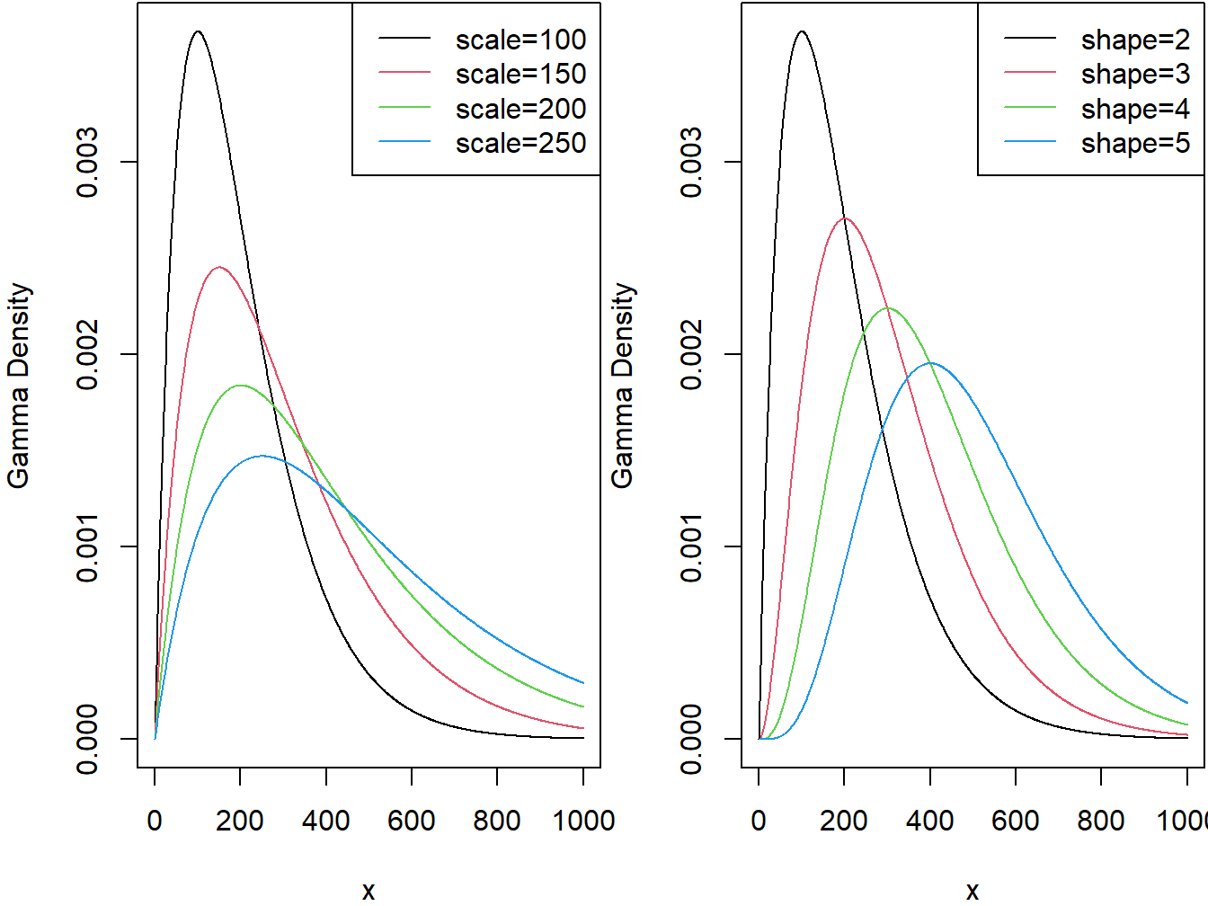
Figure 4.1: Gamma Densities. The left-hand panel is with shape=2 and varying scale. The right-hand panel is with scale=100 and varying shape.

R Code for Gamma Density Plots

par(mfrow = c(1, 2), mar = c(4, 4, 0.1, 0.1))

# Varying Scale Gamma Densities
scaleparam <- seq(100, 250, by = 50)
shapeparam <- 2:5
x <- seq(0, 1000, by = 1)
fgamma <- dgamma(x, shape = 2, scale = scaleparam[1])
plot(x, fgamma, type = "l", ylab = "Gamma Density")
for (k in 2:length(scaleparam)) {
    fgamma <- dgamma(x, shape = 2, scale = scaleparam[k])
    lines(x, fgamma, col = k)
}
legend("topright", c("scale=100", "scale=150", "scale=200", "scale=250"), lty = 1,
    col = 1:4)

# Varying Shape Gamma Densities
fgamma <- dgamma(x, shape = shapeparam[1], scale = 100)
plot(x, fgamma, type = "l", ylab = "Gamma Density")
for (k in 2:length(shapeparam)) {
    fgamma <- dgamma(x, shape = shapeparam[k], scale = 100)
    lines(x, fgamma, col = k)
}
legend("topright", c("shape=2", "shape=3", "shape=4", "shape=5"), lty = 1, col = 1:4)

When \(\alpha = 1\) the gamma reduces to an exponential distributionA single parameter continous probability distribution that is defined by its rate parameter and when \(\alpha = \frac{n}{2}\) and \(\theta = 2\) the gamma reduces to a chi-square distributionA common distribution used in chi-square tests for determining goodness of fit of observed data to a theorized distribution with \(n\) degrees of freedom. As we will see in Section 17.4, the chi-square distribution is used extensively in statistical hypothesis testing.

The distribution function of the gamma model is the incomplete gamma function, denoted by \(\Gamma\left(\alpha; \frac{x}{\theta} \right)\), and defined as \[ F_{X}\left( x \right) = \Gamma\left( \alpha; \frac{x}{\theta} \right) = \frac{1}{\Gamma\left( \alpha \right)}\int_{0}^{x /\theta}t^{\alpha - 1}e^{- t}~dt , \] with \(\alpha > 0,\ \theta > 0\). For an integer \(\alpha\), it can be written as \(\Gamma\left( \alpha; \frac{x}{\theta} \right) = 1 - e^{-x/\theta}\sum_{k = 0}^{\alpha-1}\frac{(x/\theta)^k}{k!}\).

The \(k\)-th raw moment of the gamma distributed random variable for any positive \(k\) is given by \[ \mathrm{E}\left( X^{k} \right) = \theta^{k} \frac{\Gamma\left( \alpha + k \right)}{\Gamma\left( \alpha \right)} . \] The mean and variance are given by \(\mathrm{E}\left( X \right) = \alpha\theta\) and \(\mathrm{Var}\left( X \right) = \alpha\theta^{2}\), respectively.

Since all moments exist for any positive \(k\), the gamma distribution is considered a light tailed distributionA distribution with thinner tails than the benchmark exponential distribution, which may not be suitable for modeling risky assets as it will not provide a realistic assessment of the likelihood of severe losses.

4.2.2 Pareto Distribution

The Pareto distributionA heavy-tailed and positively skewed distribution with 2 parameters, named after the Italian economist Vilfredo Pareto (1843-1923), has many economic and financial applications. It is a positively skewed and heavy-tailed distribution which makes it suitable for modeling income, high-risk insurance claims and severity of large casualty losses. The survival function of the Pareto distribution which decays slowly to zero was first used to describe the distribution of income where a small percentage of the population holds a large proportion of the total wealth. For extreme insurance claims, the tail of the severity distribution (losses in excess of a threshold) can be modeled using a Generalized Pareto distribution.

The continuous variable \(X\) is said to have the (two parameter) Pareto distribution with shape parameter \(\alpha\) and scale parameter \(\theta\) if its pdfProbability density function is given by

\[\begin{equation} f_{X}\left( x \right) = \frac{\alpha\theta^{\alpha}}{\left( x + \theta \right)^{\alpha + 1}} \ \ \ x > 0, \ \alpha > 0, \ \theta > 0. \tag{4.1} \end{equation}\]

The two panels in Figure 4.2 demonstrate the effect of the scale and shape parameters on the Pareto density function. There are other formulations of the Pareto distribution including a one parameter version given in Appendix Section 20.2. Henceforth, when we refer the Pareto distribution, we mean the version given through the pdf in equation (4.1).

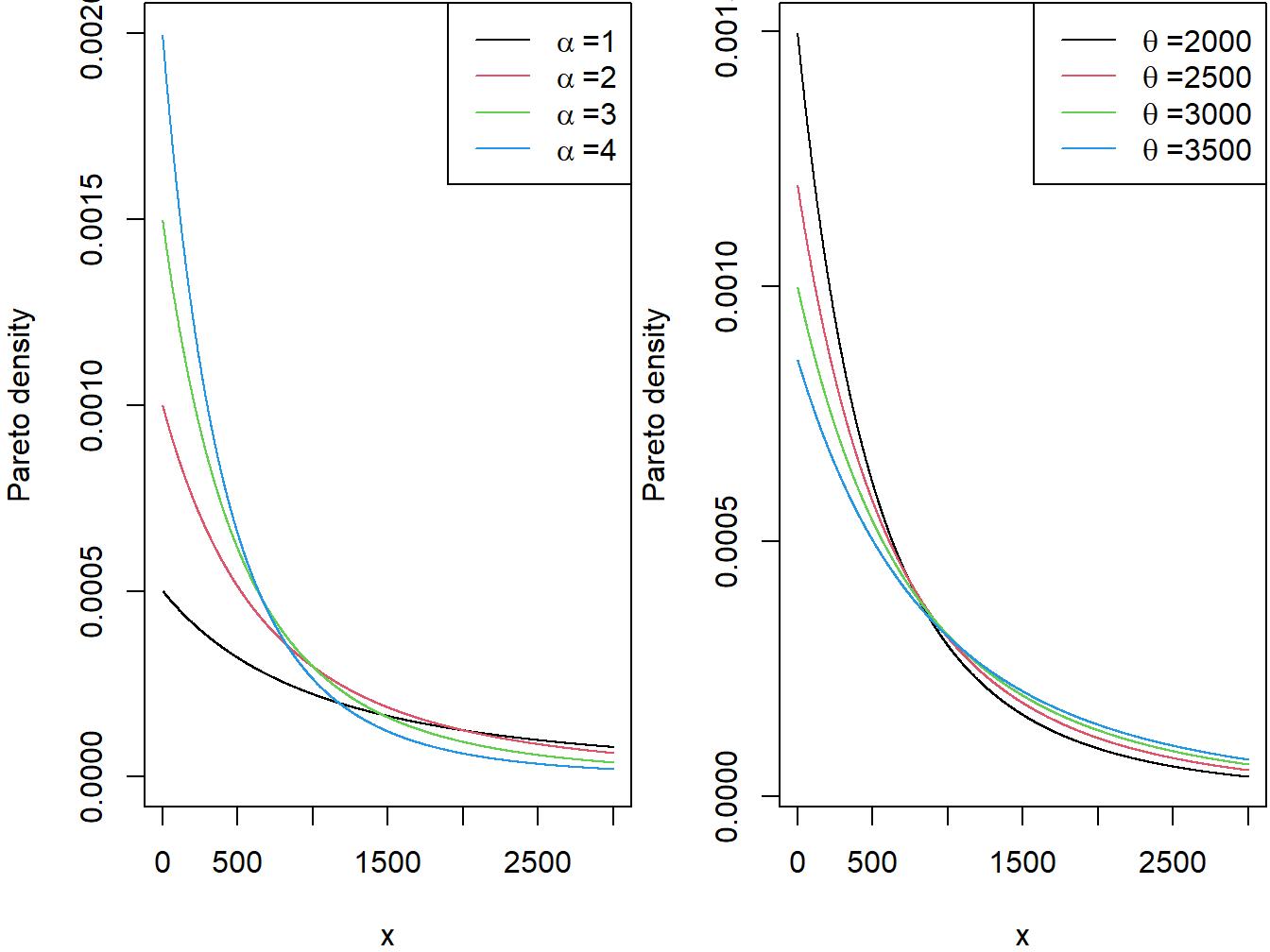
Figure 4.2: Pareto Densities. The left-hand panel is with scale=2000 and varying shape. The right-hand panel is with shape=3 and varying scale.

R Code for Pareto Density Plots

par(mfrow = c(1, 2), mar = c(4, 4, 0.1, 0.1))

# Varying Scale Pareto Densities
x <- seq(1, 3000, by = 1)
scaleparam <- seq(2000, 3500, 500)
shapeparam <- 1:4

# varying the shape parameter
plot(x, actuar::dpareto(x, shape = shapeparam[1], scale = 2000), ylim = c(0, 0.002),
    type = "l", ylab = "Pareto density")
for (k in 2:length(shapeparam)) {
    lines(x, actuar::dpareto(x, shape = shapeparam[k], scale = 2000), col = k)
}
legend("topright", c(expression(alpha ~ "=1"), expression(alpha ~ "=2"), expression(alpha ~
    "=3"), expression(alpha ~ "=4")), lty = 1, col = 1:4)

# Varying Shape Pareto Densities
plot(x, actuar::dpareto(x, shape = 3, scale = scaleparam[1]), type = "l", ylab = "Pareto density")
for (k in 2:length(scaleparam)) {
    lines(x, actuar::dpareto(x, shape = 3, scale = scaleparam[k]), col = k)
}
legend("topright", c(expression(theta ~ "=2000"), expression(theta ~ "=2500"), expression(theta ~
    "=3000"), expression(theta ~ "=3500")), lty = 1, col = 1:4)

The distribution function of the Pareto distribution is given by \[ F_{X}\left( x \right) = 1 - \left( \frac{\theta}{x + \theta} \right)^{\alpha} \ \ \ x > 0,\ \alpha > 0,\ \theta > 0. \]

It can be easily seen that the hazard functionRatio of the probability density function and the survival function: f(x)/s(x), and represents an instantaneous probability within a small time frame of the Pareto distribution is a decreasing function in \(x\), another indication that the distribution is heavy tailed. Again using the analogy of the income of a population, when the hazard function decreases over time the population dies off at a decreasing rate resulting in a heavier tail for the distribution. The hazard function reveals information about the tail distribution and is often used to model data distributions in survival analysis. The hazard function is defined as the instantaneous potential that the event of interest occurs within a very narrow time frame.

The \(k\)-th raw moment of the Pareto distributed random variable exists, if and only if, \(\alpha > k\). If \(k\) is a positive integer then \[ \mathrm{E}\left( X^{k} \right) = \frac{\theta^{k}~ k!}{\left( \alpha - 1 \right)\cdots\left( \alpha - k \right)} \ \ \ \alpha > k. \] The mean and variance are given by \[\mathrm{E}\left( X \right) = \frac{\theta}{\alpha - 1} \ \ \ \text{for } \alpha > 1\] and \[\mathrm{Var}\left( X \right) = \frac{\alpha\theta^{2}}{\left( \alpha - 1 \right)^{2}\left( \alpha - 2 \right)} \ \ \ \text{for } \alpha > 2,\]respectively.

Example 4.2.1. The claim size of an insurance portfolio follows the Pareto distribution with mean and variance of 40 and 1800, respectively. Find

1. The shape and scale parameters.
2. The 95-th percentile of this distribution.

Show Example Solution

Solution.

a. As, \(X\sim Pa(\alpha,\theta)\), we have \(\mathrm{E}\left( X \right) = \frac{\theta}{\alpha - 1} = 40\) and \(\mathrm{Var}\left( X \right) = \frac{\alpha\theta^{2}}{\left( \alpha - 1 \right)^{2}\left( \alpha - 2 \right)} = 1800\). By dividing the square of the first equation by the second we get \(\frac{\alpha - 2}{\alpha} = \frac{40^{2}}{1800}\). Thus, \(\alpha = 18.02\) and \(\theta = 680.72\).
b. The 95-th percentile, \(\pi_{0.95}\), satisfies the equation \[ F_{X}\left( \pi_{0.95} \right) = 1 - \left( \frac{680.72}{\pi_{0.95} + 680.72} \right)^{18.02} = 0.95. \] Thus, \(\pi_{0.95} = 122.96\).

---

4.2.3 Weibull Distribution

The Weibull distributionA positively skewed continuous distribution with 2 parameters that can have an increasing or decreasing hazard function depending on the shape parameter, named after the Swedish physicist Waloddi Weibull (1887-1979) is widely used in reliability, life data analysis, weather forecasts and general insurance claims. Truncated data arise frequently in insurance studies. The Weibull distribution has been used to model excess of loss treaty over automobile insurance as well as earthquake inter-arrival times.

The continuous variable \(X\) is said to have the Weibull distribution with shape parameter \(\alpha\) and scale parameter \(\theta\) if its pdf is given by \[ f_{X}\left( x \right) = \frac{\alpha}{\theta}\left( \frac{x}{\theta} \right)^{\alpha - 1} \exp \left(- \left( \frac{x}{\theta} \right)^{\alpha}\right) \ \ \ x > 0,\ \alpha > 0,\ \theta > 0. \] The two panels in Figure 4.3 demonstrate the effects of the scale and shape parameters on the Weibull density function.

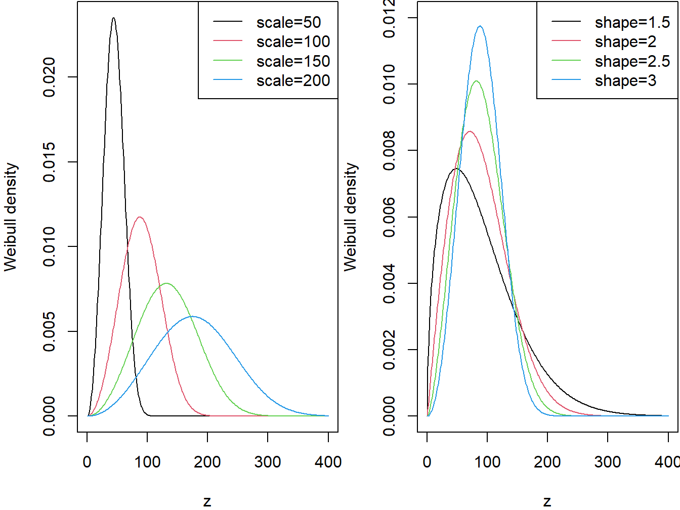
Figure 4.3: Weibull Densities. The left-hand panel is with shape=3 and varying scale. The right-hand panel is with scale=100 and varying shape.

R Code for Weibull Density Plots

par(mfrow = c(1, 2), mar = c(4, 4, 0.1, 0.1))

# Varying Scale Weibull Densities
z <- seq(0, 400, by = 1)
scaleparam <- seq(50, 200, 50)
shapeparam <- seq(1.5, 3, 0.5)
plot(z, dweibull(z, shape = 3, scale = scaleparam[1]), type = "l", ylab = "Weibull density")
for (k in 2:length(scaleparam)) {
    lines(z, dweibull(z, shape = 3, scale = scaleparam[k]), col = k)
}
legend("topright", c("scale=50", "scale=100", "scale=150", "scale=200"), lty = 1,
    col = 1:4)

# Varying Shape Weibull Densities
plot(z, dweibull(z, shape = shapeparam[1], scale = 100), ylim = c(0, 0.012), type = "l",
    ylab = "Weibull density")
for (k in 2:length(shapeparam)) {
    lines(z, dweibull(z, shape = shapeparam[k], scale = 100), col = k)
}
legend("topright", c("shape=1.5", "shape=2", "shape=2.5", "shape=3"), lty = 1, col = 1:4)

The distribution function of the Weibull distribution is given by \[ F_{X}\left( x \right) = 1 - \exp\left(- \left( \frac{x}{\theta} \right)^{\alpha}~\right) \ \ \ x > 0,\ \alpha > 0,\ \theta > 0. \]

It can be easily seen that the shape parameter \(\alpha\) describes the shape of the hazard function of the Weibull distribution. The hazard function is a decreasing function when \(\alpha < 1\) (heavy tailed distribution), constant when \(\alpha = 1\) and increasing when \(\alpha > 1\) (light tailed distribution). This behavior of the hazard function makes the Weibull distribution a suitable model for a wide variety of phenomena such as weather forecasting, electrical and industrial engineering, insurance modeling, and financial risk analysis.

The \(k\)-th raw moment of the Weibull distributed random variable is given by \[ \mathrm{E}\left( X^{k} \right) = \theta^{k}~\Gamma\left( 1 + \frac{k}{\alpha} \right) . \]

The mean and variance are given by \[ \mathrm{E}\left( X \right) = \theta~\Gamma\left( 1 + \frac{1}{\alpha} \right) \] and \[ \mathrm{Var}(X)= \theta^{2}\left( \Gamma\left( 1 + \frac{2}{\alpha} \right) - \left\lbrack \Gamma\left( 1 + \frac{1}{\alpha} \right) \right\rbrack ^{2}\right), \] respectively.

Example 4.2.2. Suppose that the probability distribution of the lifetime of AIDS patients (in months) from the time of diagnosis is described by the Weibull distribution with shape parameter 1.2 and scale parameter 33.33.

1. Find the probability that a randomly selected person from this population survives at least 12 months.
2. A random sample of 10 patients will be selected from this population. What is the probability that at most two will die within one year of diagnosis.
3. Find the 99-th percentile of the distribution of lifetimes.

Show Example Solution

Solution.

a. Let \(X\) be the lifetime of AIDS patients (in months) having a Weibull distribution with parameters \(\left( 1.2,33.33 \right)\). We have,

\[ \Pr \left( X \geq 12 \right) = S_{X} \left( 12 \right) = e^{- \left( \frac{12}{33.33} \right)^{1.2}} = 0.746. \]

b. Let \(Y\) be the number of patients who die within one year of diagnosis. Then, \(Y\sim Bin\left( 10,\ 0.254 \right)\) and \(\Pr\left( Y \leq 2 \right) = 0.514.\)

c. Let \(\pi_{0.99}\) denote the 99-th percentile of this distribution. Then, \[ S_{X}\left( \pi_{0.99} \right) = \exp\left\{- \left( \frac{\pi_{0.99}}{33.33} \right)^{1.2}\right\} = 0.01. \] Solving for \(\pi_{0.99}\), we get \(\pi_{0.99} = 118.99\).

---

4.2.4 The Generalized Beta Distribution of the Second Kind

The Generalized Beta Distribution of the Second KindA 4-parameter flexible distribution that encompasses many common distributions (GB2) was introduced by G. Venter (1983) in the context of insurance loss modeling and by McDonald (1984) as an income and wealth distribution. It is a four-parameter, very flexible, distribution that can model positively as well as negatively skewed distributions.

The continuous variable \(X\) is said to have the GB2 distribution with parameters \(\sigma\), \(\theta\), \(\alpha_1\) and \(\alpha_2\) if its pdf is given by

\[\begin{equation} f_{X}\left( x \right) = \frac{(x/\theta)^{\alpha_2/\sigma}}{x \sigma~\mathrm{B}\left( \alpha_1,\alpha_2\right)\left\lbrack 1 + \left( x/\theta \right)^{1/\sigma} \right\rbrack^{\alpha_1 + \alpha_2}} \ \ \ \text{for } x > 0, \tag{4.2} \end{equation}\]

\(\sigma,\theta,\alpha_1,\alpha_2 > 0\), and where the beta function \(\mathrm{B}\left( \alpha_1,\alpha_2 \right)\) is defined as

\[ \mathrm{B}\left( \alpha_1,\alpha_2\right) = \int_{0}^{1}{t^{\alpha_1 - 1}\left( 1 - t \right)^{\alpha_2 - 1}}~ dt. \]

The GB2 provides a model for heavy as well as light tailed data. It includes the exponential, gamma, Weibull, Burr, Lomax, F, chi-square, Rayleigh, lognormal and log-logistic as special or limiting cases. For example, by setting the parameters \(\sigma = \alpha_1 = \alpha_2 = 1\), the GB2 reduces to the log-logistic distribution. When \(\sigma = 1\) and \(\alpha_2 \rightarrow \infty\), it reduces to the gamma distribution, and when \(\alpha = 1\) and \(\alpha_2 \rightarrow \infty\), it reduces to the Weibull distribution.

A GB2 random variable can be constructed as follows. Suppose that \(G_1\) and \(G_2\) are independent random variables where \(G_i\) has a gamma distribution with shape parameter \(\alpha_i\) and scale parameter 1. Then, one can show that the random variable \(X = \theta \left(\frac{G_1}{G_2}\right)^{\sigma}\) has a GB2 distribution with pdf summarized in equation (4.2). This theoretical result has several implications. For example, when the moments exist, one can show that the \(k\)-th raw moment of the GB2 distributed random variable is given by

\[ \mathrm{E}\left( X^{k} \right) = \frac{\theta^{k}~\mathrm{B}\left( \alpha_1 +k \sigma,\alpha_2 - k \sigma \right)}{\mathrm{B}\left( \alpha_1,\alpha_2 \right)}, \ \ \ k > 0. \]

As will be described in Section 4.3.1.2, the GB2 is also related to an \(F\)-distribution, a result that can be useful in simulation and residual analysis.

Earlier applications of the GB2 were on income data and more recently have been used to model long-tailed claims data (Section 13.2 describes different interpretations of the descriptor “long-tail”). The GB2 has been used to model different types of automobile insurance claims, severity of fire losses, as well as medical insurance claim data.

Show Quiz Solution

---

4.3 Methods of Creating New Distributions

---

In this section, you learn how to:

• Understand connections among the distributions
• Give insights into when a distribution is preferred when compared to alternatives
• Provide foundations for creating new distributions

---

4.3.1 Functions of Random Variables and their Distributions

In Section 4.2 we discussed some elementary known distributions. In this section we discuss means of creating new parametric probability distributions from existing ones. Specifically, let \(X\) be a continuous random variable with a known pdf \(f_{X}(x)\) and distribution function \(F_{X}(x)\). We are interested in the distribution of \(Y = g\left( X \right)\), where \(g(X)\) is a one-to-one transformationA function or method that turns one distribution into another defining a new random variable \(Y\). In this section we apply the following techniques for creating new families of distributions: (a) multiplication by a constant (b) raising to a power, (c) exponentiation and (d) mixing.

4.3.1.1 Multiplication by a Constant

If claim data show change over time then such transformation can be useful to adjust for inflation. If the level of inflation is positive then claim costs are rising, and if it is negative then costs are falling. To adjust for inflation we multiply the cost \(X\) by 1+ inflation rate (negative inflation is deflation). To account for currency impact on claim costs we also use a transformation to apply currency conversion from a base to a counter currency.

Consider the transformation \(Y = cX\), where \(c > 0\), then the distribution function of \(Y\) is given by \[ F_{Y}\left( y \right) = \Pr\left( Y \leq y \right) = \Pr\left( cX \leq y \right) = \Pr\left( X \leq \frac{y}{c} \right) = F_{X}\left( \frac{y}{c} \right). \] Using the chain rule for differentiation, the pdf of interest \(f_{Y}(y)\) can be written as \[ f_{Y}\left( y \right) = \frac{1}{c}f_{X}\left( \frac{y}{c} \right). \] Suppose that \(X\) belongs to a certain set of parametric distributionsProbability distribution defined by a fixed set of parameters and define a rescaled version \(Y\ = \ cX\), \(c\ > \ 0\). If \(Y\) is in the same set of distributions then the distribution is said to be a scale distributionA distribution with the property that multiplying all values by a constant leads to the same distribution family with only the scale parameter changed. When a member of a scale distribution is multiplied by a constant \(c\) (\(c > 0\)), the scale parameter for this scale distribution meets two conditions:

• The parameter is changed by multiplying by \(c\);
• All other parameters remain unchanged.

Example 4.3.1. Actuarial Exam Question. Losses of Eiffel Auto Insurance are denoted in Euro currency and follow a lognormal distribution with \(\mu = 8\) and \(\sigma = 2\). Given that 1 euro \(=\) 1.3 dollars, find the set of lognormal parameters which describe the distribution of Eiffel’s losses in dollars.

Show Example Solution

Solution.

Let \(X\) and \(Y\) denote the aggregate losses of Eiffel Auto Insurance in euro currency and dollars respectively. As \(Y = 1.3X\), we have, \[ F_{Y}\left( y \right) = \Pr\left( Y \leq y \right) = \Pr\left( 1.3X \leq y \right) = \Pr\left( X \leq \frac{y}{1.3} \right) = F_{X}\left( \frac{y}{1.3} \right). \]

\(X\) follows a lognormal distribution with parameters \(\mu = 8\) and \(\sigma = 2\). The pdf of \(X\) is given by \[ f_{X}\left( x \right) = \frac{1}{x \sigma \sqrt{2\pi}}\exp \left\{- \frac{1}{2}\left( \frac{\log x - \mu}{\sigma} \right)^{2}\right\} \ \ \ \text{for } x > 0. \] As \(\left| \frac{dx}{dy} \right| = \frac{1}{1.3}\), the pdf of interest \(f_{Y}(y)\) is

\[ \begin{array}{ll} f_{Y}\left( y \right) & = \frac{1}{1.3}f_{X}\left( \frac{y}{1.3} \right) \\ &= \frac{1}{1.3}\frac{1.3}{y \sigma \sqrt{2\pi}}\exp \left\{- \frac{1}{2}\left( \frac{\log\left( y/1.3 \right) - \mu}{\sigma} \right)^{2}\right\} \\ &= \frac{1}{y \sigma\sqrt{2\pi}}\exp \left\{- \frac{1}{2}\left( \frac{\log y - \left( \log 1.3 + \mu \right)}{\sigma} \right)^{2}\right\}. \end{array} \] Then \(Y\) follows a lognormal distribution with parameters \(\log 1.3 + \mu = 8.26\) and \(\sigma = 2.00\). If we let \(\mu = \log(m)\) then it can be easily seen that \(m = e^{\mu}\) is the scale parameter which was multiplied by 1.3 while \(\sigma\) is the shape parameter that remained unchanged.

---

Example 4.3.2. Actuarial Exam Question. Demonstrate that the gamma distribution is a scale distribution.

Show Example Solution

Solution.

Let \(X\sim Ga(\alpha,\theta)\) and \(Y = cX\). As \(\left| \frac{dx}{dy} \right| = \frac{1}{c}\), then

\[ f_{Y}\left( y \right) = \frac{1}{c}f_{X}\left( \frac{y}{c} \right) = \frac{\left( \frac{y}{c\theta} \right)^{\alpha}}{y~\Gamma\left( \alpha \right)}\exp \left( - \frac{y}{c\theta} \right) . \] We can see that \(Y\sim Ga(\alpha,c\theta)\) indicating that gamma is a scale distribution and \(\theta\) is a scale parameter.

Using the same approach you can demonstrate that other distributions introduced in Section 4.2 are also scale distributions. In actuarial modeling, working with a scale distribution is very convenient because it allows to incorporate the effect of inflation and to accommodate changes in the currency unit.

---

4.3.1.2 Raising to a Power

In Section 4.2.3 we talked about the flexibility of the Weibull distribution in fitting reliability dataA dataset consisting of failure times for failed units and run times for units still functioning. Looking to the origins of the Weibull distribution, we recognize that the Weibull is a power transformationA transformation type that involves raising a random variable to a power of the exponential distribution. This is an application of another type of transformation which involves raising the random variable to a power.

Consider the transformation \(Y = X^{\tau}\), where \(\tau > 0\), then the distribution function of \(Y\) is given by

\[ F_{Y}\left( y \right) = \Pr\left( Y \leq y \right) = \Pr\left( X^{\tau} \leq y \right) = \Pr\left( X \leq y^{1/ \tau} \right) = F_{X}\left( y^{1/ \tau} \right). \]

Hence, the pdf of interest \(f_{Y}(y)\) can be written as \[ f_{Y}(y) = \frac{1}{\tau} y^{(1/ \tau) - 1} f_{X}\left( y^{1/ \tau} \right). \] On the other hand, if \(\tau < 0\), then the distribution function of \(Y\) is given by \[ F_{Y}\left( y \right) = \Pr\left( Y \leq y \right) = \Pr\left( X^{\tau} \leq y \right) = \Pr\left( X \geq y^{1/ \tau} \right) = 1 - F_{X}\left( y^{1/ \tau} \right), \] and

\[ f_{Y}(y) = \left| \frac{1}{\tau} \right|{y^{(1/ \tau) - 1}f}_{X}\left( y^{1/ \tau} \right). \]

Example 4.3.3. We assume that \(X\) follows the exponential distribution with mean \(\theta\) and consider the transformed variable \(Y = X^{\tau}\). Show that \(Y\) follows the Weibull distribution when \(\tau\) is positive and determine the parameters of the Weibull distribution.

Show Example Solution

Solution.

As \(X\) follows the exponential distribution with mean \(\theta\), we have \[ f_{X}(x) = \frac{1}{\theta}e^{- x/ \theta} \ \ \ \, x > 0. \] Solving for x yields \(x = y^{1/\tau}\). Taking the derivative, we have

\[ \left| \frac{dx}{dy} \right| = \frac{1}{\tau}{y^{\frac{1}{\tau}-1}}. \] Thus,

\[ f_{Y}\left( y \right) = \frac{1}{\tau}{y^{\frac{1}{\tau} - 1}f}_{X}\left( y^{\frac{1}{\tau}} \right) \\ = \frac{1}{\tau \theta }y^{\frac{1}{\tau} - 1}e^{- \frac{y^{\frac{1}{\tau}}}{\theta}} = \frac{\alpha}{\beta}\left( \frac{y}{\beta} \right)^{\alpha - 1}e^{- \left( y/ \beta \right)^{\alpha}}. \] where \(\alpha = \frac{1}{\tau}\) and \(\beta = \theta^{\tau}\). Then, \(Y\) follows the Weibull distribution with shape parameter \(\alpha\) and scale parameter \(\beta\).

---

Special Case. Relating a GB2 to an \(F\)- Distribution. We can use tranforms such as multiplication by a constant and raising to a power to verify that the GB2 distribution is related to an \(F\)-distribution, a distribution widely used in applied statistics.

Relating a GB2 to an F- Distribution

---

To see this relationship, we first note that \(\frac{1}{2} G_1\) has a gamma distribution with shape parameter \(\alpha_1\) and scale parameter \(0.5\). Readers with some background in applied statistics may also recognize this to be a chi-square distribution with degrees of freedom \(2\alpha_1\). The ratio of independent chi-squares has an \(F\)-distribution. That is

\[ \frac{G_1}{G_2} = \frac{0.5G_1}{0.5G_2} = F \]

has an \(F\)-distribution with numerator degrees of freedom \(2\alpha_1\) and denominator degrees of freedom \(2\alpha_2\). Thus, a random variable \(X\) with a GB2 distribution can be expressed as \(X = \theta \left(\frac{G_1}{G_2}\right)^{\sigma}= \theta ~ F^{\sigma}\). With this, you can think of a GB2 as a “power \(F\)” or a “generalized \(F\),” as it is sometimes known in the literature.

Simulation, discussed in Chapter 8, provides a direct application of this result. Suppose we know how to simulate an outcome with an \(F-distribution\) (that is easy to do using, for example, the R function rf(n,df1,df2)), say \(F\). Then we raise it to the power \(\sigma\) and multiply it by \(\theta\) so that \(\theta ~ F^{\sigma}\) is an outcome that has a GB2 distribution.

Residual analysis provides another direct application. Suppose we have an outcome, say \(X\), that we think comes from a GB2 distribution. Then we can examine the transformed version \(X^{\ast} = \left(X/\theta\right)^{1/\sigma}\). If the original specification is correct, then \(X^{\ast}\) has an \(F-\) distribution and there are many well-known techniques, some described in Chapter 6, for verifying this assertion.

---

4.3.1.3 Exponentiation

The normal distribution is a very popular model for a wide number of applications and when the sample size is large, it can serve as an approximate distribution for other models. If the random variable \(X\) has a normal distribution with mean \(\mu\) and variance \(\sigma^{2}\), then \(Y = e^{X}\) has a lognormal distributionA heavy-tailed, positively skewed 2-parameter continuous distribution such that the natural log of the random variable is normally distributed with the same parameter values with parameters \(\mu\) and \(\sigma^{2}\). The lognormal random variable has a lower bound of zero, is positively skewed and has a long right tail. A lognormal distribution is commonly used to describe distributions of financial assets such as stock prices. It is also used in fitting claim amounts for automobile as well as health insurance. This is an example of another type of transformation which involves exponentiation.

In general, consider the transformation \(Y = e^{X}\). Then, the distribution function of \(Y\) is given by

\[ F_{Y}\left( y \right) = \Pr\left( Y \leq y \right) = \Pr\left( e^{X} \leq y \right) = \Pr\left( X \leq \log y \right) = F_{X}\left( \log y \right). \] Taking derivatives, we see that the pdf of interest \(f_{Y}(y)\) can be written as \[ f_{Y}(y) = \frac{1}{y}f_{X}\left( \log y \right). \] As an important special case, suppose that \(X\) is normally distributed with mean \(\mu\) and variance \(\sigma^2\). Then, the distribution of \(Y = e^X\) is

\[ f_{Y}(y) = \frac{1}{y}f_{X}\left( \log y \right) = \frac{1}{y \sigma \sqrt{2 \pi}} \exp \left\{-\frac{1}{2}\left(\frac{ \log y - \mu}{\sigma}\right)^2\right\}. \] This is known as a lognormal distribution.

Example 4.3.4. Actuarial Exam Question. Assume that \(X\) has a uniform distribution on the interval \((0,\ c)\) and define \(Y = e^{X}\). Find the distribution of \(Y\).

Show Example Solution

Solution.

We begin with the cdfCumulative distribution function of \(Y\), \[ F_{Y}\left( y \right) = \Pr\left( Y \leq y \right) = \Pr\left( e^{X} \leq y \right) = \Pr\left( X \leq \log y \right) = F_{X}\left( \log y \right). \] Taking the derivative, we have,

\[ f_{Y}\left( y \right) = \frac{1}{y}f_{X}\left(\log y \right) = \frac{1}{cy} . \] Since \(0 < x < c\), then \(1 < y < e^{c}\).

---

4.3.2 Mixture Distributions for Severity

Mixture distributions represent a useful way of modeling data that are drawn from a heterogeneous populationA dataset where the subpopulations are represented by separate distinct distributions. This parent population can be thought to be divided into multiple subpopulations with distinct distributions.

4.3.2.1 Finite Mixtures

4.3.2.1.1 Two-point Mixture

If the underlying phenomenon is diverse and can actually be described as two phenomena representing two subpopulations with different modes, we can construct the two-point mixture random variable \(X\). Given random variables \(X_{1}\) and \(X_{2}\), with pdfs \(f_{X_{1}}\left( x \right)\) and \(f_{X_{2}}\left( x \right)\) respectively, the pdf of \(X\) is the weighted average of the component pdf \(f_{X_{1}}\left( x \right)\) and \(f_{X_{2}}\left( x \right)\). The pdf and distribution function of \(X\) are given by \[f_{X}\left( x \right) = af_{X_{1}}\left( x \right) + \left( 1 - a \right)f_{X_{2}}\left( x \right),\] and \[F_{X}\left( x \right) = aF_{X_{1}}\left( x \right) + \left( 1 - a \right)F_{X_{2}}\left( x \right),\]

for \(0 < a <1\), where the mixing parametersProportion weight given to each subpopulation in a mixture \(a\) and \((1 - a)\) represent the proportions of data points that fall under each of the two subpopulations respectively. This weighted average can be applied to a number of other distribution related quantities. The k-th raw moment and moment generating function of \(X\) are given by \(\mathrm{E}\left( X^{k} \right) = a\mathrm{E}\left( X_{1}^{K} \right) + \left( 1 - a \right)\mathrm{E}\left( X_{2}^{k} \right)\), and \[M_{X}(t) = aM_{X_{1}}(t) + \left( 1 - a \right)M_{X_{2}}(t),\] respectively.

Example 4.3.5. Actuarial Exam Question. A collection of insurance policies consists of two types. 25% of policies are Type 1 and 75% of policies are Type 2. For a policy of Type 1, the loss amount per year follows an exponential distribution with mean 200, and for a policy of Type 2, the loss amount per year follows a Pareto distribution with parameters \(\alpha=3\) and \(\theta=200\). For a policy chosen at random from the entire collection of both types of policies, find the probability that the annual loss will be less than 100, and find the average loss.

Show Example Solution

Solution.

The two types of losses are the random variables \(X_1\) and \(X_2\). \(X_1\) has an exponential distribution with mean 100, so \(F_{X_1}\left(100\right)=1-e^{-\frac{100}{200}}=0.393\). \(X_2\) has a Pareto distribution with parameters \(\alpha=3\) and \(\theta=200\), so \(F_{X_1}\left(100\right)=1-\left(\frac{200}{100+200}\right)^3=0.704\). Hence, \(F_X\left(100\right)=\left(0.25\times0.393\right)+\left(0.75\times0.704\right)=0.626\).

The average loss is given by \[\mathrm{E}\left(X\right)=0.25\mathrm{E}\left(X_1\right)+0.75\mathrm{E}\left(X_2\right)=\left(0.25\times200\right)+\left(0.75\times100\right)=125\].

---

4.3.2.1.2 k-point Mixture

In case of finite mixture distributions, the random variable of interest \(X\) has a probability \(p_{i}\) of being drawn from homogeneous subpopulation \(i\), where \(i = 1,2,\ldots,k\) and \(k\) is the initially specified number of subpopulations in our mixture. The mixing parameter \(p_{i}\) represents the proportion of observations from subpopulation \(i\). Consider the random variable \(X\) generated from \(k\) distinct subpopulations, where subpopulation \(i\) is modeled by the continuous distribution \(f_{X_{i}}\left( x \right)\). The probability distribution of \(X\) is given by \[f_{X}\left( x \right) = \sum_{i = 1}^{k}{p_{i}f_{X_{i}}\left( x \right)},\] where \(0 < p_{i} < 1\) and \(\sum_{i = 1}^{k} p_{i} = 1\).

This model is often referred to as a finite mixtureA mixture distribution with a finite k number of subpopulations or a \(k\)-point mixture. The distribution function, \(r\)-th raw moment and moment generating functions of the \(k\)-th point mixture are given as

\[F_{X}\left( x \right) = \sum_{i = 1}^{k}{p_{i}F_{X_{i}}\left( x \right)},\] \[\mathrm{E}\left( X^{r} \right) = \sum_{i = 1}^{k}{p_{i}\mathrm{E}\left( X_{i}^{r} \right)}, \ \ \ \text{and}\] \[M_{X}(t) = \sum_{i = 1}^{k}{p_{i}M_{X_{i}}(t)},\] respectively.

Example 4.3.6. Actuarial Exam Question. \(Y_{1}\) is a mixture of \(X_{1}\) and \(X_{2}\) with mixing weights \(a\) and \((1 - a)\). \(Y_{2}\) is a mixture of \(X_{3}\) and \(X_{4}\) with mixing weights \(b\) and \((1 - b)\). \(Z\) is a mixture of \(Y_{1}\) and \(Y_{2}\) with mixing weights \(c\) and \((1 - c)\).

Show that \(Z\) is a mixture of \(X_{1}\), \(X_{2}\), \(X_{3}\) and \(X_{4}\), and find the mixing weights.

Show Example Solution

Solution. Applying the formula for a mixed distribution, we get \[f_{Y_{1}}\left( x \right) = af_{X_{1}}\left( x \right) + \left( 1 - a \right)f_{X_{2}}\left( x \right)\]

\[f_{Y_{2}}\left( x \right) = bf_{X_{3}}\left( x \right) + \left( 1 - b \right)f_{X_{4}}\left( x \right)\]

\[f_{Z}\left( x \right) = cf_{Y_{1}}\left( x \right) + \left( 1 - c \right)f_{Y_{2}}\left( x \right)\]

Substituting the first two equations into the third, we get

\[f_{Z}\left( x \right) = c\left\lbrack af_{X_{1}}\left( x \right) + \left( 1 - a \right)f_{X_{2}}\left( x \right) \right\rbrack + \left( 1 - c \right)\left\lbrack bf_{X_{3}}\left( x \right) + \left( 1 - b \right)f_{X_{4}}\left( x \right) \right\rbrack\]

\[= caf_{X_{1}}\left( x \right) + c\left( 1 - a \right)f_{X_{2}}\left( x \right) + \left( 1 - c \right)bf_{X_{3}}\left( x \right) + (1 - c)\left( 1 - b \right)f_{X_{4}}\left( x \right)\].

Then, \(Z\) is a mixture of \(X_{1}\), \(X_{2}\), \(X_{3}\) and \(X_{4}\), with mixing weights \(\text{ca}\), \(c\left( 1 - a \right)\), \(\left( 1 - c \right)b\) and \((1 - c)\left( 1 - b \right)\), respectively. It can be easily seen that the mixing weights sum to one.

---

4.3.2.2 Continuous Mixtures

A mixture with a very large number of subpopulations (\(k\) goes to infinity) is often referred to as a continuous mixtureA mixture distribution with an infinite number of subpopulations, where the mixing parameter is itself a continuous distribution. In a continuous mixture, subpopulations are not distinguished by a discrete mixing parameter but by a continuous variable \(\Theta\), where \(\Theta\) plays the role of \(p_{i}\) in the finite mixture. Consider the random variable \(X\) with a distribution depending on a parameter \(\Theta\), where \(\Theta\) itself is a continuous random variable. This description yields the following model for \(X\) \[ f_{X}\left( x \right) = \int_{-\infty}^{\infty}{f_{X}\left(x \left| \theta \right. \right)g_{\Theta}( \theta )} d \theta , \] where \(f_{X}\left( x | \theta \right)\) is the conditional distributionA probability distribution that applies to a subpopulation satisfying the condition of \(X\) at a particular value of \(\Theta=\theta\) and \(g_{\Theta}\left( \theta \right)\) is the probability statement made about the unknown parameter \(\theta\). In a Bayesian context (described in Section ??), this is known as the prior distributionA probability distribution assigned prior to observing additional data of \(\Theta\) (the prior information or expert opinion to be used in the analysis).

The distribution function, \(k\)-th raw moment and moment generating functions of the continuous mixture are given as

\[ F_{X}\left( x \right) = \int_{-\infty}^{\infty}{F_{X}\left(x \left| \theta \right. \right) g_{\Theta}(\theta)} d \theta, \] \[ \mathrm{E}\left( X^{k} \right) = \int_{-\infty}^{\infty}{\mathrm{E}\left( X^{k}\left| \theta \right. \right)g_{\Theta}(\theta)}d \theta, \] \[ M_{X}(t) = \mathrm{E}\left( e^{t X} \right) = \int_{-\infty}^{\infty}{\mathrm{E}\left( e^{ tx}\left| \theta \right. \right)g_{\Theta}(\theta)}d \theta, \] respectively.

The \(k\)-th raw moment of the mixture distribution can be rewritten as \[ \mathrm{E}\left( X^{k} \right) = \int_{-\infty}^{\infty}{\mathrm{E}\left( X^{k}\left| \theta \right. \right)g_{\Theta}(\theta)}d\theta ~=~ \mathrm{E}\left\lbrack \mathrm{E}\left( X^{k}\left| \Theta \right. \right) \right\rbrack . \]

Using the law of iterated expectations (see Appendix Chapter 18), we can define the mean and variance of \(X\) as \[ \mathrm{E}\left( X \right) = \mathrm{E}\left\lbrack \mathrm{E}\left( X\left| \Theta \right. \right) \right\rbrack \] and \[ \mathrm{Var}\left( X \right) = \mathrm{E}\left\lbrack \mathrm{Var}\left( X\left| \Theta \right. \right) \right\rbrack + \mathrm{Var}\left\lbrack \mathrm{E}\left( X\left| \Theta \right. \right) \right\rbrack . \]

Example 4.3.7. Actuarial Exam Question. \(X\) has a normal distribution with a mean of \(\Lambda\) and variance of 1. \(\Lambda\) has a normal distribution with a mean of 1 and variance of 1. Find the mean and variance of \(X\).

Show Example Solution

Solution.

X is a continuous mixture with mean

\[ \mathrm{E}\left(X\right)=\mathrm{E}\left[\mathrm{E}\left(X\middle|\Lambda\right)\right]=\mathrm{E}\left(\Lambda\right)=1 \text{ and } \mathrm{V}\left(X\right)=\mathrm{V}\left[\mathrm{E}\left(X\middle|\Lambda\right)\right]+\mathrm{E}\left[\mathrm{V}\left(X\middle|\Lambda\right)\right]=\mathrm{V}\left(\Lambda\right)+\mathrm{E}\left(1\right)=1+1=2. \]

---

Example 4.3.8. Actuarial Exam Question. Claim sizes, \(X\), are uniform on the interval \(\left(\Theta,\Theta+10\right)\) for each policyholder. \(\Theta\) varies by policyholder according to an exponential distribution with mean 5. Find the unconditional distributionA probability distribution independent of any another imposed conditions, mean and variance of \(X\).

Show Example Solution

Solution.

The conditional distribution of \(X\) is \(f_{X}\left( x | \theta \right) = \frac{1}{10}\) for \(\theta < x < \theta + 10\). The prior distribution of \(\theta\) is \(g_{\Theta}(\theta) = \frac{1}{5}e^{- \frac{\theta}{5}}\) for \(0 < \theta < \infty\).

Multiplying and integrating yields the unconditional distribution of \(X\)

\[ f_{X}\left( x \right) = \int f_{X}\left( x |\theta \right) ~g_{\Theta}(\theta) d \theta . \]

For this example, this is

\[ f_{X}\left( x \right) = \left\{ \begin{matrix} \int_{0}^{x}{\frac{1}{50}e^{- \frac{\theta}{5}}d\theta = \frac{1}{10}\left( 1 - e^{- \frac{x}{5}} \right)} & 0 \leq x \leq 10, \\ \int_{x - 10}^{x}{\frac{1}{50}e^{- \frac{\theta}{5}} d\theta} = \frac{1}{10}\left( e^{- \frac{\left( x - 10 \right)}{5}} - e^{- \frac{x}{5}} \right) & 10 < x < \infty. \\ \end{matrix} \right.\ \]

One can use this to derive the mean and variance of the unconditional distribution. Alternatively, start with the conditional mean and variance of \(X\), given by

\[ \mathrm{E}\left( X | \theta \right)= \frac{\theta + \theta + 10}{2} = \theta + 5 \] and \[ \mathrm{Var}\left( X | \theta \right)= \frac{\left\lbrack \left( \theta + 10 \right) - \theta \right\rbrack^{2}}{12} = \frac{100}{12}, \] respectively. With these, the unconditional mean and variance of \(X\) are given by

\[ \mathrm{E}\left( X \right) = \mathrm{E}\left\lbrack \mathrm{E}\left( X\left| \Theta \right. \right) \right\rbrack = \mathrm{E}\left( \Theta + 5 \right) = \mathrm{E}\left( \Theta \right) + 5 = 5 + 5 = 10, \]

and

\[ \mathrm{Var}\left( X \right) = \mathrm{E}\left\lbrack V\left( X\left| \Theta \right. \right) \right\rbrack + \mathrm{Var}\left\lbrack \mathrm{E}\left( X\left| \Theta \right. \right) \right\rbrack \\ = \mathrm{E}\left( \frac{100}{12} \right) + \mathrm{Var}\left( \Theta + 5 \right) = 8.33 + \mathrm{Var}\left( \Theta \right) = 33.33. \]

---

Show Quiz Solution

---

4.4 Estimating Loss Distributions

---

In this section, you learn how to:

• Estimate moments, quantiles, and distributions without reference to a parametric distribution
• Summarize the data graphically without reference to a parametric distribution
• Use method of moments, percentile matching, and maximum likelihood estimation to estimate parameters for different distributions.

---

4.4.1 Nonparametric Estimation

In Section 3.2 for frequency and Section 4.1 for severity, we learned how to summarize a distribution by computing means, variances, quantiles/percentiles, and so on. To approximate these summary measures using a dataset, one strategy is to:

1. assume a parametric form for a distribution, such as a negative binomial for frequency or a gamma distribution for severity,
2. estimate the parameters of that distribution, and then
3. use the distribution with the estimated parameters to calculate the desired summary measure.

This is the parametricDistributional assumptions made on the population from which the data is drawn, with properties defined using parameters. approach. Another strategy is to estimate the desired summary measure directly from the observations without reference to a parametric model. Not surprisingly, this is known as the nonparametricNo distributional assumptions are made on the population from which the data is drawn. approach.

Let us start by considering the most basic type of sampling schemeHow the data is obtained from the population and what data is observed. and assume that observations are realizations from a set of random variables \(X_1, \ldots, X_n\) that are iidIndependent and identically distributed draws from an unknown population distribution \(F(\cdot)\). An equivalent way of saying this is that \(X_1, \ldots, X_n\), is a random sample (with replacement) from \(F(\cdot)\). We now describe nonparametric estimators of many important measures that summarize a distribution.

4.4.1.1 Moment Estimators

We learned how to define moments in Section 3.2.2 for frequency and Section 4.1.1 for severity. In particular, the \(k\)-th moment, \(\mathrm{E~}[X^k] = \mu^{\prime}_k\), summarizes many aspects of the distribution for different choices of \(k\). Here, \(\mu^{\prime}_k\) is sometimes called the \(k\)th population moment to distinguish it from the \(k\)th sample moment, \[ \frac{1}{n} \sum_{i=1}^n X_i^k , \] which is the corresponding nonparametric estimator. In typical applications, \(k\) is a positive integer, although it need not be in theory. The sample estimator for the population mean \(\mu\) is called the sample mean, denoted with a bar on top of the random variable:

\[ \overline{X} =\frac{1}{n} \sum_{i=1}^n X_i . \] A nonparametric, or sample, estimator of the \(k\)-th central moment, \(\mu_k\) is \[ \frac{1}{n} \sum_{i=1}^n \left(X_i - \overline{X}\right)^k . \] Properties of the sample moment estimator of the variance such as \(n^{-1}\sum_{i=1}^n \left(X_i - \overline{X}\right)^2\) have been studied extensively but is not the only possible estimator. The most widely used version is one where the effective sample size is reduced by one, and so we define \[ s^2 = \frac{1}{n-1} \sum_{i=1}^n \left(X_i - \overline{X}\right)^2. \]

Dividing by \(n-1\) instead of \(n\) matters little when you have a large sample size \(n\) as is common in insurance applications. The sample variance estimator \(s^2\) is unbiasedAn estimator that has no bias, that is, the expected value of an estimator equals the parameter being estimated. in the sense that \(\mathrm{E~} [s^2] = \sigma^2\), a desirable property particularly when interpreting results of an analysis.

4.4.1.2 Empirical Distribution Function

We have seen how to compute nonparametric estimators of the \(k\)th moment \(\mathrm{E~} [X^k]\). In the same way, for any known function \(\mathrm{g}(\cdot)\), we can estimate \(\mathrm{E~} [\mathrm{g}(X)]\) using \(n^{-1}\sum_{i=1}^n \mathrm{g}(X_i)\).

Now consider the function \(\mathrm{g}(X) = I(X \le x)\) for a fixed \(x\). Here, the notation \(I(\cdot)\) is the indicatorA categorical variable that has only two groups. the numerical values are usually taken to be one to indicate the presence of an attribute, and zero otherwise. another name for a binary variable. function; it returns 1 if the event \((\cdot)\) is true and 0 otherwise. Note that now the random variable \(\mathrm{g}(X)\) has Bernoulli distribution (a binomial distribution with \(n=1\)). We can use this distribution to readily calculate quantities such as the mean and the variance. For example, for this choice of \(\mathrm{g}(\cdot)\), the expected value is \(\mathrm{E~} [I(X \le x)] = \Pr(X \le x) = F(x)\), the distribution function evaluated at \(x\). Using the analog principle, we define the nonparametric estimator of the distribution function

\[ \begin{aligned} F_n(x) &= \frac{1}{n} \sum_{i=1}^n I\left(X_i \le x\right) \\ &= \frac{\text{number of observations less than or equal to }x}{n} . \end{aligned} \] As \(F_n(\cdot)\) is based on only observations and does not assume a parametric family for the distribution, it is nonparametric and also known as the empirical distribution functionThe empirical distribution is a non-parametric estimate of the underlying distribution of a random variable. it directly uses the data observations to construct the distribution, with each observed data point in a size-n sample having probability 1/n. . It is also known as the empirical cumulative distribution function and, in R, one can use the ecdf(.) function to compute it.

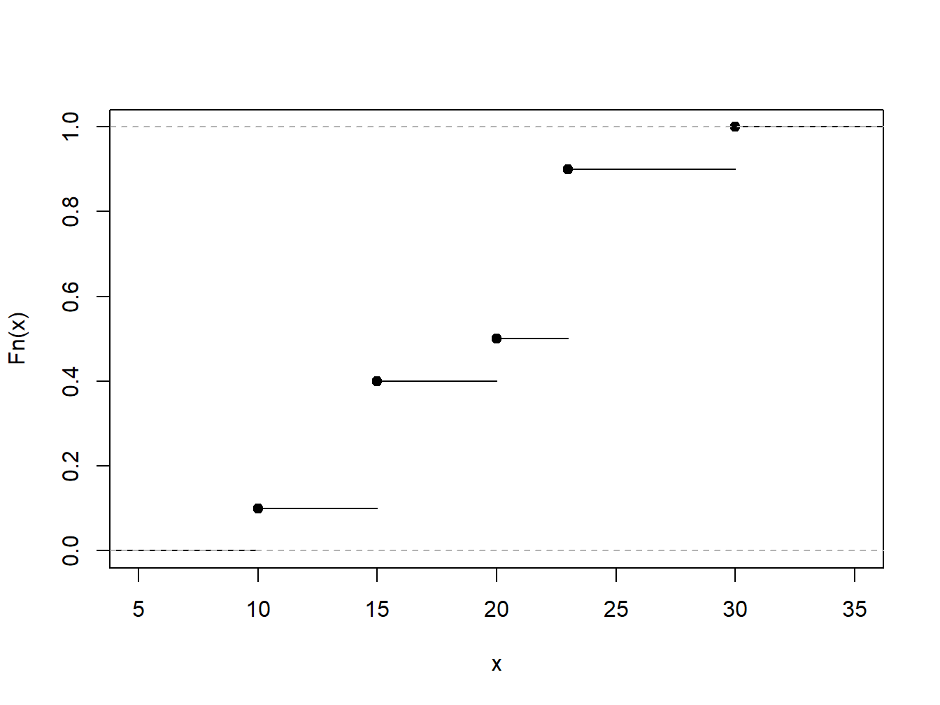
Example 4.4.1. Toy Data Set. To illustrate, consider a fictitious, or “toy,” data set of \(n=10\) observations. Determine the empirical distribution function.

\[ {\small \begin{array}{c|cccccccccc} \hline i &1&2&3&4&5&6&7&8&9&10 \\ X_i& 10 &15 &15 &15 &20 &23 &23 &23 &23 &30\\ \hline \end{array} } \]

Show Example Solution

You should check that the sample mean is \(\overline{X} = 19.7\) and that the sample variance is \(s^2 =34.45556\). The corresponding empirical distribution function is

\[ \begin{aligned} F_n(x) &= \left\{ \begin{array}{ll} 0 & \text{ for }\ x<10 \\ 0.1 & \text{ for }\ 10 \leq x<15 \\ 0.4 & \text{ for }\ 15 \leq x<20 \\ 0.5 & \text{ for }\ 20 \leq x<23 \\ 0.9 & \text{ for }\ 23 \leq x<30 \\ 1 & \text{ for }\ x \geq 30, \end{array} \right.\end{aligned} \]

as shown in Figure 4.4. The empirical distribution is generally discrete and continuous from the right.

Figure 4.4: Empirical Distribution Function of a Toy Example

Show R Code

(xExample <- c(10, rep(15, 3), 20, rep(23, 4), 30))
PercentilesxExample <- ecdf(xExample)
plot(PercentilesxExample, main = "", xlab = "x")

4.4.1.3 Quartiles, Percentiles and Quantiles

We have already seen in Section 4.1.2 the median50th percentile of a definition, or middle value where half of the distribution lies below, which is the number such that approximately half of a data set is below (or above) it. The first quartileThe 25th percentile; the number such that approximately 25% of the data is below it. is the number such that approximately 25% of the data is below it and the third quartileThe 75th percentile; the number such that approximately 75% of the data is below it. is the number such that approximately 75% of the data is below it. A \(100p\) percentileA 100p-th percentile is the number such that 100 times p percent of the data is below it. is the number such that \(100 \times p\) percent of the data is below it.

To generalize this concept, consider a distribution function \(F(\cdot)\), which may or may not be continuous, and let \(q\) be a fraction so that \(0<q<1\). We want to define a quantileThe q-th quantile is the point(s) at which the distribution function is equal to q, i.e. the inverse of the cumulative distribution function., say \(q_F\), to be a number such that \(F(q_F) \approx q\). Notice that when \(q = 0.5\), \(q_F\) is the median; when \(q = 0.25\), \(q_F\) is the first quartile, and so on. In the same way, when \(q = 0, 0.01, 0.02, \ldots, 0.99, 1.00\), the resulting \(q_F\) is a percentile. So, a quantile generalizes the concepts of median, quartiles, and percentiles.

To be precise, for a given \(0<q<1\), define the \(q\)th quantile \(q_F\) to be any number that satisfies

\[\begin{equation} F(q_F-) \le q \le F(q_F) \tag{4.3} \end{equation}\]

Here, the notation \(F(x-)\) means to evaluate the function \(F(\cdot)\) as a left-hand limit.

To get a better understanding of this definition, let us look at a few special cases. First, consider the case where \(X\) is a continuous random variable so that the distribution function \(F(\cdot)\) has no jump points, as illustrated in Figure 4.5. In this figure, a few fractions, \(q_1\), \(q_2\), and \(q_3\) are shown with their corresponding quantiles \(q_{F,1}\), \(q_{F,2}\), and \(q_{F,3}\). In each case, it can be seen that \(F(q_F-)= F(q_F)\) so that there is a unique quantile. Because we can find a unique inverse of the distribution function at any \(0<q<1\), we can write \(q_F= F^{-1}(q)\).

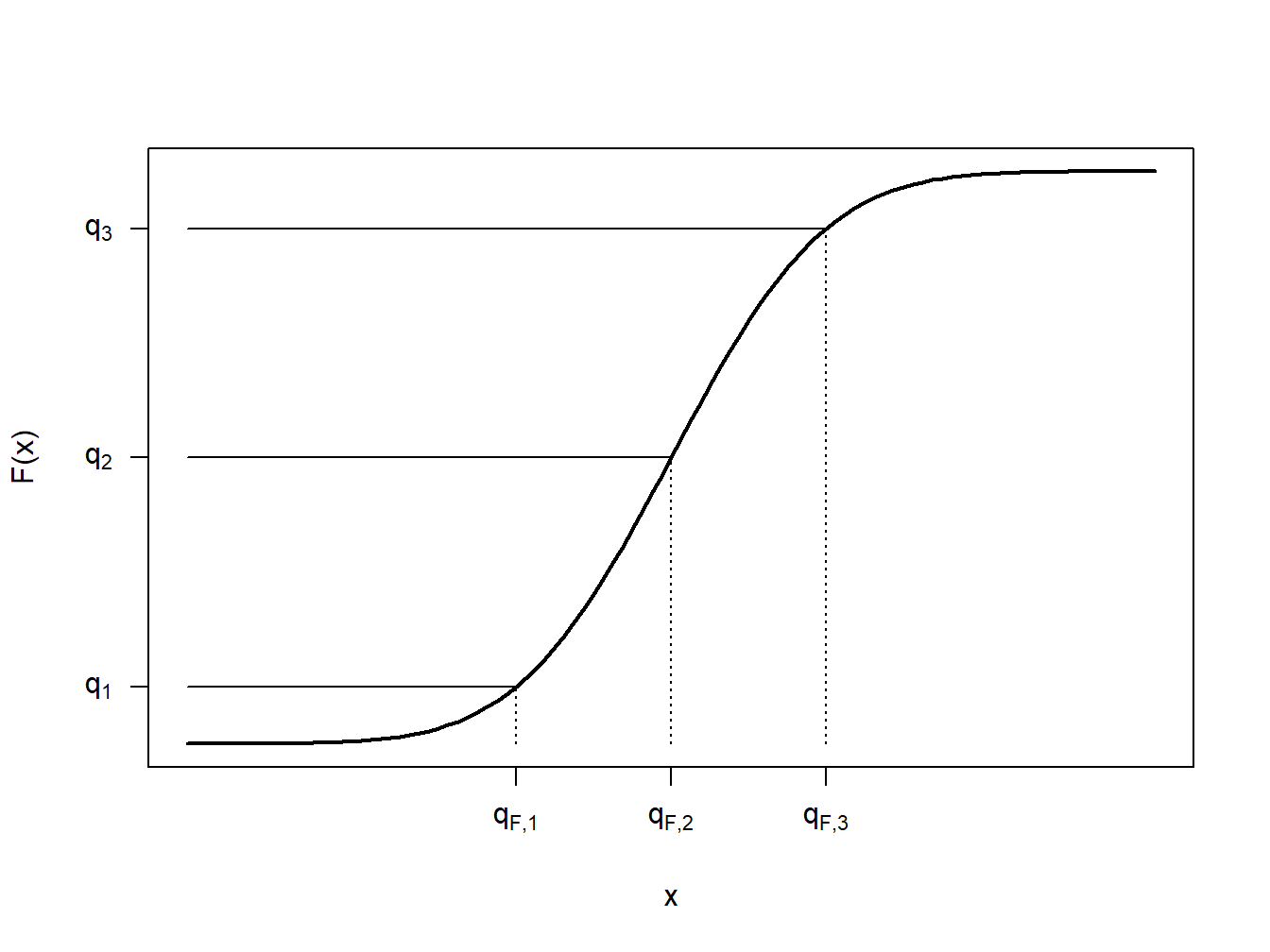
Figure 4.5: Continuous Quantile Case

Figure 4.6 shows three cases for distribution functions. The left panel corresponds to the continuous case just discussed. The middle panel displays a jump point similar to those we already saw in the empirical distribution function of Figure 4.4. For the value of \(q\) shown in this panel, we still have a unique value of the quantile \(q_F\). Even though there are many values of \(q\) such that \(F(q_F-) \le q \le F(q_F)\), for a particular value of \(q\), there is only one solution to equation (4.3). The right panel depicts a situation in which the quantile cannot be uniquely determined for the \(q\) shown as there is a range of \(q_F\)’s satisfying equation (4.3).

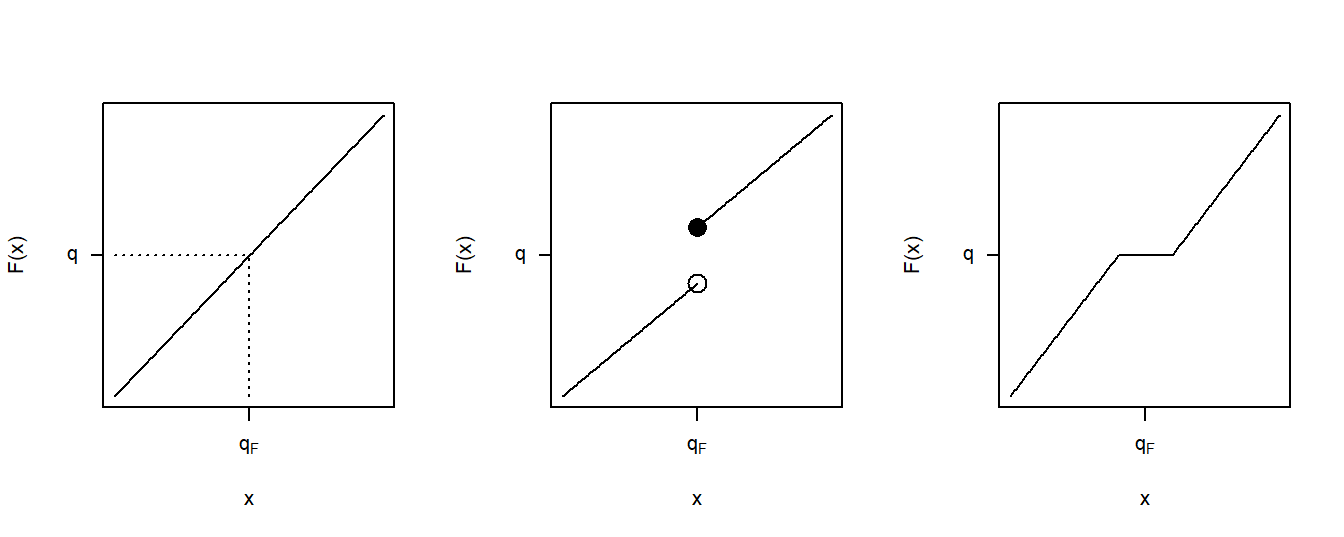
Figure 4.6: Three Quantile Cases

---

Example 4.4.2. Toy Data Set: Continued. Determine quantiles corresponding to the 20th, 50th, and 95th percentiles.

Show Example Solution

Solution. Consider Figure 4.4. The case of \(q=0.20\) corresponds to the middle panel of Figure Figure 4.6, so the 20th percentile is 15. The case of \(q=0.50\) corresponds to the right panel, so the median is any number between 20 and 23 inclusive. Many software packages use the average 21.5 (e.g. R, as seen below). For the 95th percentile, the solution is 30. We can see from Figure 4.4 that 30 also corresponds to the 99th and the 99.99th percentiles.

xExample <- c(10, rep(15, 3), 20, rep(23, 4), 30)
quantile(xExample, probs = c(0.2, 0.5, 0.95), type = 6)

 20%  50%  95% 
15.0 21.5 30.0 

---

By taking a weighted average between data observations, smoothed empirical quantiles can handle cases such as the right panel in Figure 4.6. The \(q\)th smoothed empirical quantileA quantile obtained by linear interpolation between two empirical quantiles, i.e. data points. is defined as \[ \hat{\pi}_q = (1-h) X_{(j)} + h X_{(j+1)} \] where \(j=\lfloor(n+1)q\rfloor\), \(h=(n+1)q-j\), and \(X_{(1)}, \ldots, X_{(n)}\) are the ordered values (known as the order statistics) corresponding to \(X_1, \ldots, X_n\). (Recall that the brackets \(\lfloor \cdot\rfloor\) are the floor function denoting the greatest integer value.) Note that \(\hat{\pi}_q\) is simply a linear interpolation between \(X_{(j)}\) and \(X_{(j+1)}\).

Example 4.4.3. Toy Data Set: Continued. Determine the 50th and 20th smoothed percentiles.

Show Example Solution

Solution Take \(n=10\) and \(q=0.5\). Then, \(j=\lfloor(11)(0.5) \rfloor= \lfloor 5.5 \rfloor=5\) and \(h=(11)(0.5)-5=0.5\). Then the 0.5-th smoothed empirical quantile is \[\hat{\pi}_{0.5} = (1-0.5) X_{(5)} + (0.5) X_{(6)} = 0.5 (20) + (0.5)(23) = 21.5.\] Now take \(n=10\) and \(q=0.2\). In this case, \(j=\lfloor(11)(0.2)\rfloor=\lfloor 2.2 \rfloor=2\) and \(h=(11)(0.2)-2=0.2\). Then the 0.2-th smoothed empirical quantile is \[\hat{\pi}_{0.2} = (1-0.2) X_{(2)} + (0.2) X_{(3)} = 0.8 (15) + (0.2)(15) = 15.\]

---

4.4.1.4 Density Estimators

Discrete Variable. When the random variable is discrete, estimating the probability mass function \(f(x) = \Pr(X=x)\) is straightforward. We simply use the sample average, defined to be

\[ f_n(x) = \frac{1}{n} \sum_{i=1}^n I(X_i = x), \]

which is the proportion of the sample equal to \(x\).

Continuous Variable within a Group. For a continuous random variable, consider a discretized formulation in which the domain of \(F(\cdot)\) is partitioned by constants \(\{c_0 < c_1 < \cdots < c_k\}\) into intervals of the form \([c_{j-1}, c_j)\), for \(j=1, \ldots, k\). The data observations are thus “grouped” by the intervals into which they fall. Then, we might use the basic definition of the empirical mass function, or a variation such as \[f_n(x) = \frac{n_j}{n \times (c_j - c_{j-1})} \ \ \ \ \ \ c_{j-1} \le x < c_j,\] where \(n_j\) is the number of observations (\(X_i\)) that fall into the interval \([c_{j-1}, c_j)\).

Continuous Variable (not grouped). Extending this notion to instances where we observe individual data, note that we can always create arbitrary groupings and use this formula. More formally, let \(b>0\) be a small positive constant, known as a bandwidthA small positive constant that defines the width of the steps and the degree of smoothing., and define a density estimator to be

\[\begin{equation} f_n(x) = \frac{1}{2nb} \sum_{i=1}^n I(x-b < X_i \le x + b) \tag{4.4} \end{equation}\]

Show A Snippet of Theory

---

Snippet of Theory. The idea is that the estimator \(f_n(x)\) in equation (4.4) is the average over \(n\) iid realizations of a random variable with mean

\[ \begin{aligned} \mathrm{E~ } \left[\frac{1}{2b} I(x-b < X \le x + b)\right] &= \frac{1}{2b}\left(F(x+b)-F(x-b)\right) \\ & \rightarrow F^{\prime}(x) = f(x), \end{aligned} \]

as \(b\rightarrow 0\). That is, \(f_n(x)\) is an asymptotically unbiased estimator of \(f(x)\) (its expectation approaches the true value as sample size increases to infinity). This development assumes some smoothness of \(F(\cdot)\), in particular, twice differentiability at \(x\), but makes no assumptions on the form of the distribution function \(F\). Because of this, the density estimator \(f_n\) is said to be nonparametric.

---

More generally, define the kernel density estimatorA nonparametric estimator of the density function of a random variable. of the pdfProbability density function at \(x\) as

\[\begin{equation} f_n(x) = \frac{1}{nb} \sum_{i=1}^n w\left(\frac{x-X_i}{b}\right) , \tag{4.5} \end{equation}\]

where \(w\) is a probability density function centered about 0. Note that equation (4.4) is a special case of the kernel density estimator where \(w(x) = \frac{1}{2}I(-1 < x \le 1)\), also known as the uniform kernel. Other popular choices are shown in Table 4.1.

Table 4.1. Popular Kernel Choices

\[ {\small \begin{matrix} \begin{array}{l|cc} \hline \text{Kernel} & w(x) \\ \hline \text{Uniform } & \frac{1}{2}I(-1 < x \le 1) \\ \text{Triangle} & (1-|x|)\times I(|x| \le 1) \\ \text{Epanechnikov} & \frac{3}{4}(1-x^2) \times I(|x| \le 1) \\ \text{Gaussian} & \phi(x) \\ \hline \end{array}\end{matrix} } \]

Here, \(\phi(\cdot)\) is the standard normal density function. As we will see in the following example, the choice of bandwidth \(b\) comes with a bias-variance tradeoffThe tradeoff between model simplicity (underfitting; high bias) and flexibility (overfitting; high variance). between matching local distributional features and reducing the volatility.

---

Example 4.4.4. Property Fund. Figure 4.7 shows a histogram (with shaded gray rectangles) of logarithmic property claims from 2010. The (blue) thick curve represents a Gaussian kernel density where the bandwidth was selected automatically using an ad hoc rule based on the sample size and volatility of these data. For this dataset, the bandwidth turned out to be \(b=0.3255\). For comparison, the (red) dashed curve represents the density estimator with a bandwidth equal to 0.1 and the green smooth curve uses a bandwidth of 1. As anticipated, the smaller bandwidth (0.1) indicates taking local averages over less data so that we get a better idea of the local average, but at the price of higher volatility. In contrast, the larger bandwidth (1) smooths out local fluctuations, yielding a smoother curve that may miss perturbations in the local average. For actuarial applications, we mainly use the kernel density estimator to get a quick visual impression of the data. From this perspective, you can simply use the default ad hoc rule for bandwidth selection, knowing that you have the ability to change it depending on the situation at hand.

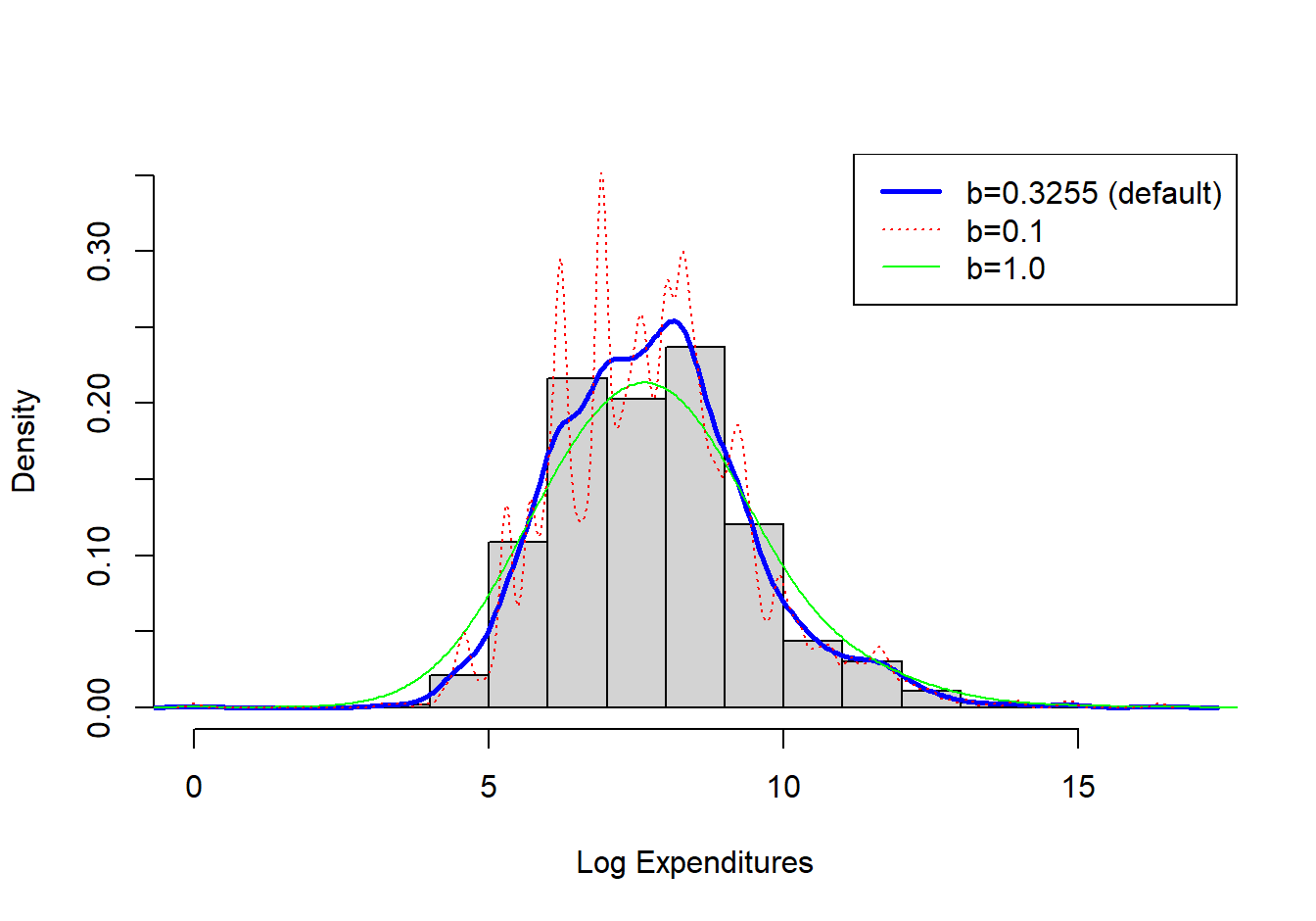
Figure 4.7: Histogram of Logarithmic Property Claims with Superimposed Kernel Density Estimators

Show R Code

ClaimLev <- read.csv("Data/CLAIMLEVEL.csv", header=TRUE); #nrow(ClaimLev); # 6258
ClaimData<-subset(ClaimLev,Year==2010);     #2010 subset
#Density Comparison
hist(log(ClaimData$Claim), main="", ylim=c(0,.35),xlab="Log Expenditures", freq=FALSE, col="lightgray")
lines(density(log(ClaimData$Claim)), col="blue",lwd=2.5)
lines(density(log(ClaimData$Claim), bw=1), col="green")
lines(density(log(ClaimData$Claim), bw=.1), col="red", lty=3)
legend("topright", c("b=0.3255 (default)", "b=0.1", "b=1.0"), lty=c(1,3,1), lwd=c(2.5,1,1),
       col=c("blue", "red", "green"), cex=1)
#density(log(ClaimData$Claim))$bw   ##default bandwidth

---

Nonparametric density estimators, such as the kernel estimator, are regularly used in practice. The concept can also be extended to give smooth versions of an empirical distribution function. Given the definition of the kernel density estimator, the kernel estimator of the distribution function can be found as

\[ \begin{aligned} \tilde{F}_n(x) = \frac{1}{n} \sum_{i=1}^n W\left(\frac{x-X_i}{b}\right).\end{aligned} \]

where \(W\) is the distribution function associated with the kernel density \(w\). To illustrate, for the uniform kernel, we have \(w(y) = \frac{1}{2}I(-1 < y \le 1)\), so

\[ \begin{aligned} W(y) = \begin{cases} 0 & y<-1\\ \frac{y+1}{2}& -1 \le y < 1 \\ 1 & y \ge 1 \\ \end{cases}\end{aligned} . \]

---

Example 4.4.5. Actuarial Exam Question.

You study five lives to estimate the time from the onset of a disease to death. The times to death are:

\[ \begin{array}{ccccc} 2 & 3 & 3 & 3 & 7 \\ \end{array} \]

Using a triangular kernel with bandwidth \(2\), calculate the density function estimate at 2.5.

Show Example Solution

Solution. For the kernel density estimate, we have \[f_n(x) = \frac{1}{nb} \sum_{i=1}^n w\left(\frac{x-X_i}{b}\right),\] where \(n=5\), \(b=2\), and \(x=2.5\). For the triangular kernel, \(w(x) = (1-|x|)\times I(|x| \le 1)\). Thus,

\[ \begin{array}{c|c|c} \hline X_i & \frac{x-X_i}{b} & w\left(\frac{x-X_i}{b} \right) \\ \hline 2 & \frac{2.5-2}{2}=\frac{1}{4} & (1-\frac{1}{4})(1) = \frac{3}{4} \\ \hline 3 & & \\ 3 & \frac{2.5-3}{2}=\frac{-1}{4} & \left(1-\left| \frac{-1}{4} \right| \right)(1) = \frac{3}{4} \\ 3 & & \\ \hline 7 & \frac{2.5-7}{2}=-2.25 & (1-|-2.25|)(0) = 0\\ \hline \end{array} \]

Then the kernel density estimate at \(x=2.5\) is \[f_n(2.5) = \frac{1}{5(2)}\left( \frac{3}{4} + (3) \frac{3}{4} + 0 \right) = \frac{3}{10}\]

---

4.4.2 Parametric Estimation

Section 4.2 has focused on parametric distributions that are commonly used in insurance applications. However, to be useful in applied work, these distributions must use “realistic” values for the parameters. In this section we cover three methods for estimating parameters: Method of moments, Percentile matching, and Maximum likelihood estimation.

4.4.2.1 Method of Moments

Under the method of momentsThe estimation of population parameters by approximating parametric moments using empirical sample moments., we approximate the moments of the parametric distribution using the empirical moments described in Section 4.4.1.1. We can then algebraically solve for the parameter estimates.

---

Example 4.4.6. Property Fund. For the 2010 property fund, there are \(n=1,377\) individual claims (in thousands of dollars) with

\[m_1 = \frac{1}{n} \sum_{i=1}^n X_i = 26.62259 \ \ \ \ \text{and} \ \ \ \ m_2 = \frac{1}{n} \sum_{i=1}^n X_i^2 = 136154.6 .\] Fit the parameters of the gamma and Pareto distributions using the method of moments.

Show Example Solution

Solution. To fit a gamma distribution, we have \(\mu_1 = \alpha \theta\) and \(\mu_2^{\prime} = \alpha(\alpha+1) \theta^2\). Equating the two yields the method of moments estimators, easy algebra shows that

\[\alpha = \frac{\mu_1^2}{\mu_2^{\prime}-\mu_1^2} \ \ \ \text{and} \ \ \ \theta = \frac{\mu_2^{\prime}-\mu_1^2}{\mu_1}.\]

Thus, the method of moment estimators are

\[ \begin{aligned} \hat{\alpha} &= \frac{26.62259^2}{136154.6-26.62259^2} = 0.005232809 \\ \hat{\theta} &= \frac{136154.6-26.62259^2}{26.62259} = 5,087.629. \end{aligned} \]

For comparison, the maximum likelihood values (see Section 4.4.2.3) turn out to be \(\hat{\alpha}_{MLE} = 0.2905959\) and \(\hat{\theta}_{MLE} = 91.61378\), so there are big discrepancies between the two estimation procedures. This is one indication, as we have seen before, that the gamma model fits poorly.

In contrast, now assume a Pareto distribution so that \(\mu_1 = \theta/(\alpha -1)\) and \(\mu_2^{\prime} = 2\theta^2/((\alpha-1)(\alpha-2) )\). Note that this expression for \(\mu_2^{\prime}\) is only valid for \(\alpha>2\). Easy algebra shows

\[\alpha = 1+ \frac{\mu_2^{\prime}}{\mu_2^{\prime}-\mu_1^2} \ \ \ \ \text{and} \ \ \ \ \ \theta = (\alpha-1)\mu_1.\]

Thus, the method of moment estimators are

\[ \begin{aligned} \hat{\alpha} &= 1+ \frac{136154.6}{136154.6-26,62259^2} = 2.005233 \\ \hat{\theta} &= (2.005233-1) \cdot 26.62259 = 26.7619 \end{aligned} \]

The maximum likelihood values turn out to be \(\hat{\alpha}_{MLE} = 0.9990936\) and \(\hat{\theta}_{MLE} = 2.2821147\). It is interesting that \(\hat{\alpha}_{MLE}<1\); for the Pareto distribution, recall that \(\alpha <1\) means that the mean is infinite. This is another indication that the property claims data set is a long tail distribution.

---

As the above example suggests, there is flexibility with the method of moments. For example, we could have matched the second and third moments instead of the first and second, yielding different estimators. Furthermore, there is no guarantee that a solution will exist for each problem. For data that are censored or truncated, matching moments is possible for a few problems but, in general, this is a more difficult scenario. Finally, for distributions where the moments do not exist or are infinite, method of moments is not available. As an alternative, one can use the percentile matching technique.

4.4.2.2 Percentile Matching

Under percentile matchingThe estimation of population parameters by approximating parametric percentiles using empirical quantiles., we approximate the quantiles or percentiles of the parametric distribution using the empirical quantiles or percentiles described in Section 4.4.1.3.

---

Example 4.4.7. Property Fund. For the 2010 property fund, we illustrate matching on quantiles. In particular, the Pareto distribution is intuitively pleasing because of the closed-form solution for the quantiles. Recall that the distribution function for the Pareto distribution is \[F(x) = 1 - \left(\frac{\theta}{x+\theta}\right)^{\alpha}.\] Easy algebra shows that we can express the quantile as

\[F^{-1}(q) = \theta \left( (1-q)^{-1/\alpha} -1 \right).\] for a fraction \(q\), \(0<q<1\).

Determine estimates of the Pareto distribution parameters using the 25th and 95th empirical quantiles.

Show Example Solution

Solution.

The 25th percentile (the first quartile) turns out to be \(0.78853\) and the 95th percentile is \(50.98293\) (both in thousands of dollars). With two equations \[0.78853 = \theta \left( 1- (1-.25)^{-1/\alpha} \right) \ \ \ \ \text{and} \ \ \ \ 50.98293 = \theta \left( 1- (1-.75)^{-1/\alpha} \right)\] and two unknowns, the solution is \[\hat{\alpha} = 0.9412076 \ \ \ \ \ \text{and} \ \ \ \ \hat{\theta} = 2.205617 .\] We remark here that a numerical routine is required for these solutions as no analytic solution is available. Furthermore, recall that the maximum likelihood estimates are \(\hat{\alpha}_{MLE} = 0.9990936\) and \(\hat{\theta}_{MLE} = 2.2821147\), so the percentile matching provides a better approximation for the Pareto distribution than the method of moments.

---

Example 4.4.8. Actuarial Exam Question. You are given:

1. Losses follow a loglogistic distribution with cumulative distribution function: \[F(x) = \frac{\left(x/\theta\right)^{\gamma}}{1+\left(x/\theta\right)^{\gamma}}\]
2. The sample of losses is:

\[ \begin{array}{ccccccccccc} 10 &35 &80 &86 &90 &120 &158 &180 &200 &210 &1500 \\ \end{array} \]

Calculate the estimate of \(\theta\) by percentile matching, using the 40th and 80th empirically smoothed percentile estimates.

Show Example Solution

Solution. With 11 observations, we have \(j=\lfloor(n+1)q\rfloor = \lfloor 12(0.4) \rfloor = \lfloor 4.8\rfloor=4\) and \(h=(n+1)q-j = 12(0.4)-4=0.8\). By interpolation, the 40th empirically smoothed percentile estimate is \(\hat{\pi}_{0.4} = (1-h) X_{(j)} + h X_{(j+1)} = 0.2(86)+0.8(90)=89.2\).

Similarly, for the 80th empirically smoothed percentile estimate, we have \(12(0.8)=9.6\) so the estimate is \(\hat{\pi}_{0.8} = 0.4(200)+0.6(210)=206\).

Using the loglogistic cumulative distribution, we need to solve the following two equations for parameters \({\hat{\theta}}\) and \({\hat{\gamma}}\): \[ 0.4=\frac{(89.2/{\hat{\theta}})^{\hat{\gamma}}}{1+(89.2/{\hat{\theta}})^{\hat{\gamma}}} \ \ \ \text{and} \ \ \ \ 0.8=\frac{(206/{\hat{\theta}})^{\hat{\gamma}}}{1+(206/{\hat{\theta}})^{\hat{\gamma}}} . \]

Solving for each parenthetical expression gives \(\frac{2}{3}=(89.2/\theta)^{\hat{\gamma}}\) and \(4=(206/{\hat{\theta}})^{\hat{\gamma}}\). Taking the ratio of the second equation to the first gives \(6=(206/89.2)^{\hat{\gamma}}\Rightarrow {\hat{\gamma}}=\frac{\log(6)}{\log(206/89.2)} = 2.1407\). Then \(4^{1/2.1407}=206/{\hat{\theta}} \Rightarrow {\hat{\theta}}=107.8\).

---

Like the method of moments, percentile matching is almost too flexible in the sense that estimators can vary depending on different percentiles chosen. For example, one actuary may use estimation on the 25th and 95th percentiles whereas another uses the 20th and 80th percentiles. In general estimated parameters will differ and there is no compelling reason to prefer one over the other. Also as with the method of moments, percentile matching is appealing because it provides a technique that can be readily applied in selected situations and has an intuitive basis. Although most actuarial applications use maximum likelihood estimators, it can be convenient to have alternative approaches such as method of moments and percentile matching available.

---

4.4.2.3 Maximum Likelihood Estimators for Complete Data

At a foundational level, we assume that the analyst has available a random sample \(X_1, \ldots, X_n\) from a distribution with distribution function \(F_X\) (for brevity, we sometimes drop the subscript \(X\)). As is common, we use the vector \(\boldsymbol \theta\) to denote the set of parameters for \(F\). This basic sample scheme is reviewed in Appendix Section 17.1. Although basic, this sampling scheme provides the foundations for understanding more complex schemes that are regularly used in practice, and so it is important to master the basics.

Before drawing from a distribution, we consider potential outcomes summarized by the random variable \(X_i\) (here, \(i\) is 1, 2, …, \(n\)). After the draw, we observe \(x_i\). Notationally, we use uppercase roman letters for random variables and lower case ones for realizations. We have seen this set-up already in Section 3.4, where we used \(\Pr(X_1 =x_1, \ldots, X_n=x_n)\) to quantify the “likelihood” of drawing a sample \(\{x_1, \ldots, x_n\}\). With continuous data, we use the joint probability density function instead of joint probabilities. With the independence assumption, the joint pdf may be written as the product of pdfs. Thus, we define the likelihood to be

\[\begin{equation} L(\boldsymbol \theta) = \prod_{i=1}^n f(x_i) . \tag{4.6} \end{equation}\]

From the notation, note that we consider this to be a function of the parameters in \(\boldsymbol \theta\), with the data \(\{x_1, \ldots, x_n\}\) held fixed. The maximum likelihood estimator is that value of the parameters in \(\boldsymbol \theta\) that maximize \(L(\boldsymbol \theta)\).

From calculus, we know that maximizing a function produces the same results as maximizing the logarithm of a function (this is because the logarithm is a monotone function). Because we get the same results, to ease computational considerations, it is common to consider the logarithmic likelihood, denoted as

\[\begin{equation} l(\boldsymbol \theta) = \log L(\boldsymbol \theta) = \sum_{i=1}^n \log f(x_i) . \tag{4.7} \end{equation}\]

Appendix Section 17.2.2 reviews the foundations of maximum likelihood estimation with more mathematical details in Appendix Chapter 19.

Example 4.4.9. Actuarial Exam Question. You are given the following five observations: 521, 658, 702, 819, 1217. You use the single-parameter Pareto with distribution function:

\[ F(x) = 1- \left(\frac{500}{x}\right)^{\alpha}, ~~~~ x>500 . \]

With \(n=5\), the log-likelihood function is \[ l(\alpha) = \sum_{i=1}^5 \log f(x_i;\alpha ) = 5 \alpha \log 500 + 5 \log \alpha -(\alpha+1) \sum_{i=1}^5 \log x_i. \]

Figure 4.8 shows the logarithmic likelihood as a function of the parameter \(\alpha\).

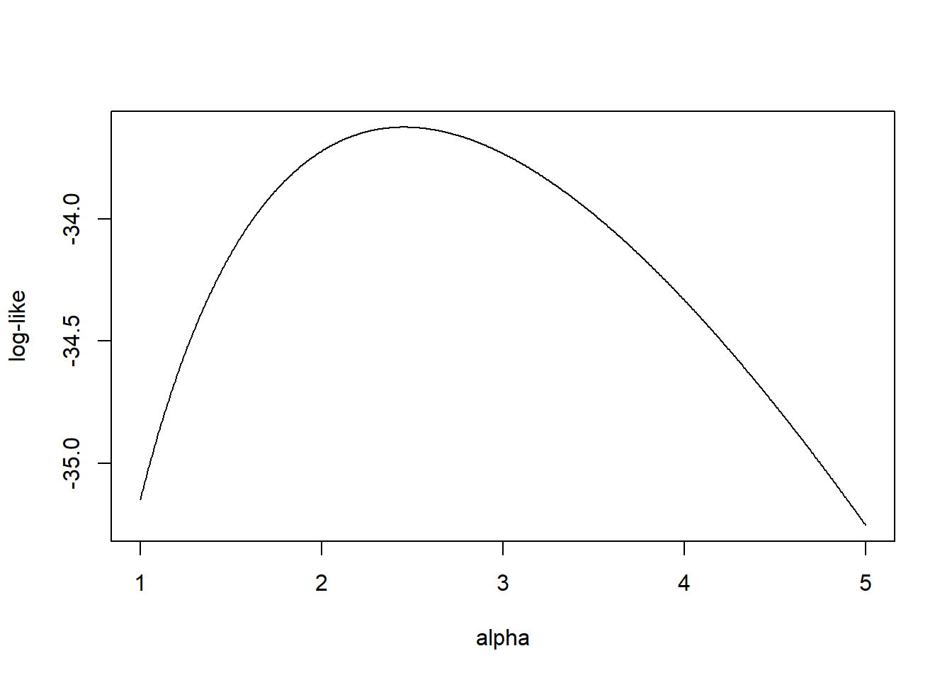
Figure 4.8: Logarithmic Likelihood for a One-Parameter Pareto

We can determine the maximum value of the logarithmic likelihood by taking derivatives and setting it equal to zero. This yields \[ \begin{array}{ll} \frac{ \partial}{\partial \alpha } l(\alpha ) &= 5 \log 500 + 5 / \alpha - \sum_{i=1}^5 \log x_i =_{set} 0 \Rightarrow \\ \hat{\alpha}_{MLE} &= \frac{5}{\sum_{i=1}^5 \log x_i - 5 \log 500 } = 2.453 . \end{array} \]

Naturally, there are many problems where it is not practical to use hand calculations for optimization. Fortunately there are many statistical routines available such as the R function optim.

R Code for Optimization

c1 <- log(521) + log(658) + log(702) + log(819) + log(1217)
nloglike <- function(alpha) {
    -(5 * alpha * log(500) + 5 * log(alpha) - (alpha + 1) * c1)
}
MLE <- optim(par = 1, fn = nloglike)$par

---

This code confirms our hand calculation result where the maximum likelihood estimator is \(\alpha_{MLE} =\) 2.453125.

---

We present a few additional examples to illustrate how actuaries fit a parametric distribution model to a set of claim data using maximum likelihood.

Example 4.4.10. Actuarial Exam Question. Consider a random sample of claim amounts: 8000 10000 12000 15000. You assume that claim amounts follow an inverse exponential distribution, with parameter \(\theta\). Calculate the maximum likelihood estimator for \(\theta\).

Show Example Solution

Solution.

The pdf is \[f_{X}\left( x \right) = \frac{\theta e^{- \frac{\theta}{x}}}{x^{2}}, \] where \(x > 0\).

The likelihood function, \(L\left( \theta \right)\), can be viewed as the probability of the observed data, written as a function of the model’s parameter \(\theta\)

\[ L\left( \theta \right) = \prod_{i = 1}^{4}{f_{X_{i}}\left( x_{i} \right)} = \frac{\theta^{4}e^{- \theta\sum_{i = 1}^{4}\frac{1}{x_{i}}}}{\prod_{i = 1}^{4}x_{i}^{2}}. \]

The log-likelihood function, \(\log L \left( \theta \right)\), is the sum of the individual logarithms

\[ \log L \left( \theta \right) = 4 \log \theta - \theta\sum_{i = 1}^{4}\frac{1}{x_{i}} - 2\sum_{i = 1}^{4}\log x_{i} . \]

Taking a derivative, we have

\[ \frac{d \log L \left( \theta \right)}{d \theta} = \frac{4}{\theta} - \sum_{i = 1}^{4}\frac{1}{x_{i}}. \]

The maximum likelihood estimator of \(\theta\), denoted by \(\hat{\theta}\), is the solution to the equation

\[ \frac{4}{\hat{\theta}} - \sum_{i = 1}^{4}{\frac{1}{x_{i}} = 0}. \]

Thus, \(\hat{\theta} = \frac{4}{\sum_{i = 1}^{4}\frac{1}{x_{i}}} = 10,667.\)

The second derivative of \(\log L \left( \theta \right)\) is given by

\[ \frac{d^{2}\log L\left( \theta \right)}{d\theta^{2}} = \frac{- 4}{\theta^{2}}. \]

Evaluating the second derivative of the loglikelihood function at \(\hat{\theta} = 10,667\) gives a negative value, indicating \(\hat{\theta}\) as the value that maximizes the loglikelihood function.

---

Example 4.4.11. Actuarial Exam Question. A random sample of size 6 is from a lognormal distribution with parameters \(\mu\) and \(\sigma\). The sample values are

\[ 200 \ \ \ 3000 \ \ \ 8000 \ \ \ 60000 \ \ \ 60000 \ \ \ 160000. \]

Calculate the maximum likelihood estimator for \(\mu\) and \(\sigma\).

Show Example Solution

Solution.

The pdf is

\[ f_{X}\left( x \right) = \frac{1}{x \sigma \sqrt{2\pi}}\exp\left( - \frac{1}{2}\left( \frac{\log x - \mu}{\sigma} \right)^{2} \right), \]

where \(x > 0\).

The likelihood function, \(L\left( \mu,\sigma \right)\), is the product of the pdf for each data point.

\[ L\left( \mu,\sigma \right) = \prod_{i = 1}^{6}{f_{X_{i}}\left( x_{i} \right)} = \frac{1}{\sigma^{6}\left( 2\pi \right)^{3}\prod_{i = 1}^{6}x_{i}}\exp\left( - \frac{1}{2}\sum_{i = 1}^{6}\left( \frac{\log x_{i} - \mu}{\sigma} \right)^{2}\right). \]

Taking a logarithm yields the loglikelihood function, \(\log L \left( \mu,\sigma \right)\), which is the sum of the individual logarithms.

\[ \log L\left( \mu,\sigma \right) = - 6 \log \sigma - 3 \log \left( 2\pi \right) - \sum_{i = 1}^{6}\log x_{i} - \frac{1}{2}\sum_{i = 1}^{6}\left( \frac{\log x_{i} - \mu}{\sigma} \right)^{2}. \]

The first partial derivatives are

\[ \begin{array}{ll} \frac{\partial \log L\left( \mu,\sigma \right)}{\partial\mu} &= \frac{1}{\sigma^{2}}\sum_{i = 1}^{6}\left( \log x_{i} - \mu \right) \\ \frac{\partial \log L\left( \mu,\sigma \right)}{\partial\sigma} &= \frac{- 6}{\sigma} + \frac{1}{\sigma^{3}}\sum_{i = 1}^{6}\left( \log x_{i} - \mu \right)^{2}. \end{array} \]

The maximum likelihood estimators of \(\mu\) and \(\sigma\), denoted by \(\hat{\mu}\) and \(\hat{\sigma}\), are the solutions to the equations

\[ \begin{array}{ll} \frac{1}{{\hat{\sigma}}^{2}}\sum_{i = 1}^{6}\left( \log x_{i} - \hat{\mu} \right) &= 0 \\ \frac{- 6}{\hat{\sigma}} + \frac{1}{{\hat{\sigma}}^{3}}\sum_{i = 1}^{6}\left( \log x_{i} - \hat{\mu} \right)^{2} &= 0 . \end{array} \]

These yield the estimates

\[ \hat{\mu} = \frac{\sum_{i = 1}^{6}{\log x_{i}}}{6} = 9.38 \ \ \ \text{and} \ \ \ {\hat{\sigma}}^{2} = \frac{\sum_{i = 1}^{6}\left( \log x_{i} - \hat{\mu} \right)^{2}}{6} = 5.12 . \]

To check that these estimates maximize, and do not minimize, the likelihood, you may also wish to compute the second partial derivatives. These are

\[ \frac{\partial^{2}\log L\left( \mu,\sigma \right)}{\partial\mu^{2}} = \frac{- 6}{\sigma^{2}}, \ \ \ \ \frac{\partial^{2}\log L\left( \mu,\sigma \right)}{\partial\mu\partial\sigma} = \frac{- 2}{\sigma^{3}}\sum_{i = 1}^{6}\left( \log x_{i} - \mu \right) \]

and

\[ \frac{\partial^{2}\log L\left( \mu,\sigma \right)}{\partial\sigma^{2}} = \frac{6}{\sigma^{2}} - \frac{3}{\sigma^{4}}\sum_{i = 1}^{6}\left( \log x_{i} - \mu \right)^{2} . \]

---

Two follow-up questions rely on large sample properties that you may have seen in an earlier course. Appendix Chapter 19 reviews the definition of the likelihood function, introduces its properties, reviews the maximum likelihood estimators, extends their large-sample properties to the case where there are multiple parameters in the model, and reviews statistical inference based on maximum likelihood estimators. In the solutions of these examples we derive the asymptotic variance of maximum-likelihood estimators of the model parameters. We use the delta method to derive the asymptotic variances of functions of these parameters.

Example 4.4.10 - Follow - Up. Refer to Example 4.4.10.

1. Approximate the variance of the maximum likelihood estimator.
2. Determine an approximate 95% confidence interval for \(\theta\).
3. Determine an approximate 95% confidence interval for \(\Pr \left( X \leq 9,000 \right).\)

Show Example Solution

Solution.

a. Taking reciprocal of negative expectation of the second derivative of \(\log L \left( \theta \right)\), we obtain an estimate of the variance of \(\hat{\theta}\), \(\widehat{Var}\left( \hat{\theta} \right) = \left. \ \left\lbrack E\left( \frac{d^{2}\log L \left( \theta \right)}{d\theta^{2}} \right) \right\rbrack^{- 1} \right|_{\theta = \hat{\theta}} = \frac{{\hat{\theta}}^{2}}{4} = 28,446,222\).

It should be noted that as the sample size \(n \rightarrow \infty\), the distribution of the maximum likelihood estimator \(\hat{\theta}\) converges to a normal distribution with mean \(\theta\) and variance \(\hat{V}\left( \hat{\theta} \right)\). The approximate confidence interval in this example is based on the assumption of normality, despite the small sample size, only for the purpose of illustration.

b. The 95% confidence interval for \(\theta\) is given by

\[ 10,667 \pm 1.96\sqrt{28,446,222} = \left( 213.34,\ 21120.66 \right). \]

c. The distribution function of \(X\) is \(F\left( x \right) = 1 - e^{- \frac{x}{\theta}}\). Then, the maximum likelihood estimate of \(g_{\Theta}(\theta) = F\left( 9,000 \right)\) is

\[ g\left( \hat{\theta} \right) = 1 - e^{- \frac{9,000}{10,667}} = 0.57. \]

We use the delta method to approximate the variance of \(g\left( \hat{\theta} \right)\). \[\frac{\text{dg}\left( \theta \right)}{d \theta} = {- \frac{9000}{\theta^{2}}e}^{- \frac{9000}{\theta}}.\]

\(\widehat{Var}\left\lbrack g\left( \hat{\theta} \right) \right\rbrack = \left( - {\frac{9000}{{\hat{\theta}}^{2}}e}^{- \frac{9000}{\hat{\theta}}} \right)^{2}\hat{V}\left( \hat{\theta} \right) = 0.0329\).

The 95% confidence interval for \(F\left( 9000 \right)\) is given by \[ 0.57 \pm 1.96\sqrt{0.0329} = \left( 0.214,\ 0.926 \right). \]

---

Example 4.4.11 - Follow - Up. Refer to Example 4.4.11.

1. Estimate the covariance matrixMatrix where the (i,j)^th element represents the covariance between the ith and jth random variables of the maximum likelihood estimator.
2. Determine approximate 95% confidence intervals for \(\mu\) and \(\sigma\).
3. Determine an approximate 95% confidence interval for the mean of the lognormal distribution.

Show Example Solution

a. To derive the covariance matrix of the mleMaximum likelihood estimate we need to find the expectations of the second derivatives. Since the random variable \(X\) is from a lognormal distribution with parameters \(\mu\) and \(\sigma\), then \(\log X\) is normally distributed with mean \(\mu\) and variance \(\sigma^{2}\).

\[ \mathrm{E}\left( \frac{\partial^{2}\text{log L}\left( \mu,\sigma \right)}{\partial\mu^{2}} \right) = \mathrm{E}\left( \frac{- 6}{\sigma^{2}} \right) = \frac{- 6}{\sigma^{2}} , \]

\[ \mathrm{E}\left( \frac{\partial^{2}\text{log L}\left( \mu,\sigma \right)}{\partial\mu\partial\sigma} \right) = \frac{- 2}{\sigma^{3}}\sum_{i = 1}^{6}{\mathrm{E}\left( \log x_{i} - \mu \right)} = \frac{- 2}{\sigma^{3}}\sum_{i = 1}^{6}\left\lbrack \mathrm{E}\left( \log x_{i} \right) - \mu \right\rbrack = \frac{- 2}{\sigma^{3}}\sum_{i = 1}^{6}\left( \mu - \mu \right) = 0, \]

and

\[ \mathrm{E}\left( \frac{\partial^{2}\text{log L}\left( \mu,\sigma \right)}{\partial\sigma^{2}} \right) = \frac{6}{\sigma^{2}} - \frac{3}{\sigma^{4}}\sum_{i = 1}^{6}{\mathrm{E}\left( \log x_{i} - \mu \right)}^{2} = \frac{6}{\sigma^{2}} - \frac{3}{\sigma^{4}}\sum_{i = 1}^{6}{\mathrm{Var}\left( \log x_{i} \right) = \frac{6}{\sigma^{2}} - \frac{3}{\sigma^{4}}\sum_{i = 1}^{6}{\sigma^{2} = \frac{- 12}{\sigma^{2}}}} . \]

Using the negatives of these expectations we obtain the Fisher information matrix

\[ \begin{bmatrix} \frac{6}{\sigma^{2}} & 0 \\ 0 & \frac{12}{\sigma^{2}} \\ \end{bmatrix}. \]

The covariance matrix, \(\Sigma\), is the inverse of the Fisher information matrix

\[ \Sigma = \begin{bmatrix} \frac{\sigma^{2}}{6} & 0 \\ 0 & \frac{\sigma^{2}}{12} \\ \end{bmatrix}. \]

The estimated matrix is given by

\[ \hat{\Sigma} = \begin{bmatrix} 0.8533 & 0 \\ 0 & 0.4267 \\ \end{bmatrix}. \]

b. The 95% confidence interval for \(\mu\) is given by \(9.38 \pm 1.96\sqrt{0.8533} = \left( 7.57,\ 11.19 \right)\).

The 95% confidence interval for \(\sigma^{2}\) is given by \(5.12 \pm 1.96\sqrt{0.4267} = \left( 3.84,\ 6.40 \right)\).

c. The mean of X is \(\exp\left( \mu + \frac{\sigma^{2}}{2} \right)\). Then, the maximum likelihood estimate of

\[ g\left( \mu,\sigma \right) = \exp\left( \mu + \frac{\sigma^{2}}{2} \right) \]

is

\[ g\left( \hat{\mu},\hat{\sigma} \right) = \exp\left( \hat{\mu} + \frac{{\hat{\sigma}}^{2}}{2} \right) = 153,277. \]

We use the delta method to approximate the variance of the mle \(g\left( \hat{\mu},\hat{\sigma} \right)\).

\(\frac{\partial g\left( \mu,\sigma \right)}{\partial\mu} = \exp\left( \mu + \frac{\sigma^{2}}{2} \right)\) and \(\frac{\partial g\left( \mu,\sigma \right)}{\partial\sigma} = \sigma \exp\left( \mu + \frac{\sigma^{2}}{2} \right)\).

Using the delta method, the approximate variance of \(g\left( \hat{\mu},\hat{\sigma} \right)\) is given by

\[ \left. \ \widehat{Var}\left( g\left( \hat{\mu},\hat{\sigma} \right) \right) = \begin{bmatrix} \frac{\partial g\left( \mu,\sigma \right)}{\partial\mu} & \frac{\partial g\left( \mu,\sigma \right)}{\partial\sigma} \\ \end{bmatrix}\Sigma\begin{bmatrix} \frac{\partial g\left( \mu,\sigma \right)}{\partial\mu} \\ \frac{\partial g\left( \mu,\sigma \right)}{\partial\sigma} \\ \end{bmatrix} \right|_{\mu = \hat{\mu},\sigma = \hat{\sigma}} \\ = \begin{bmatrix} 153,277 & 346,826 \\ \end{bmatrix}\begin{bmatrix} 0.8533 & 0 \\ 0 & 0.4267 \\ \end{bmatrix}\begin{bmatrix} 153,277 \\ 346,826 \\ \end{bmatrix} \\ = 71,374,380,000 . \]

The 95% confidence interval for \(\exp\left( \mu + \frac{\sigma^{2}}{2} \right)\) is given by

\[ 153277 \pm 1.96\sqrt{71,374,380,000} = \left( - 370356,\ 676910 \right). \]

Since the mean of the lognormal distribution cannot be negative, we should replace the negative lower limit in the previous interval by a zero.

---

Example 4.4.12. Wisconsin Property Fund. To see how maximum likelihood estimators work with real data, we return to the 2010 claims data introduced in Section 1.3.

The following snippet of code shows how to fit the exponential, gamma, Pareto, lognormal, and \(GB2\) models. For consistency, the code employs the R package VGAM. The acronym stands for Vector Generalized Linear and Additive Models; as suggested by the name, this package can do far more than fit these models although it suffices for our purposes. The one exception is the \(GB2\) density which is not widely used outside of insurance applications; however, we can code this density and compute maximum likelihood estimators using the optim general purpose optimizer.

Show Example Solution

library(VGAM)
claim_lev <- read.csv("Data/CLAIMLEVEL.csv", header = TRUE) 
claim_data <- subset(claim_lev, Year == 2010); 

# Inference assuming a GB2 Distribution - this is more complicated
# The likelihood function of GB2 distribution (negative for optimization)
lik_gb2 <- function (param) {
  a_1 <- param[1]
  a_2 <- param[2]
  mu <- param[3]
  sigma <- param[4]
  yt <- (log(claim_data$Claim) - mu) / sigma
  logexpyt <- ifelse(yt > 23, yt, log(1 + exp(yt)))
  logdens <- a_1 * yt - log(sigma) - log(beta(a_1,a_2)) - 
    (a_1+a_2) * logexpyt - log(claim_data$Claim) 
  return(-sum(logdens))
}
# "optim" is a general purpose minimization function
gb2_bop <- optim(c(1, 1, 0, 1), lik_gb2, method = c("L-BFGS-B"), 
                 lower = c(0.01, 0.01, -500, 0.01), 
                 upper = c(500, 500, 500, 500), hessian = TRUE)
# Nonparametric Plot
plot(density(log(claim_data$Claim)), main = "", xlab = "Log Expenditures",
     ylim = c(0 ,0.37))
x <- seq(0, 15, by = 0.01)
#Exponential
fit.exp <- vglm(Claim ~ 1, exponential, data = claim_data)
theta = 1 / exp(coef(fit.exp))
fexp_ex <- dgamma(exp(x), scale = exp(-coef(fit.exp)), shape = 1) * exp(x)
lines(x, fexp_ex, col = "red", lty =2)
# Inference assuming a gamma distribution
fit.gamma <- vglm(Claim ~ 1, family = gamma2, data = claim_data)
theta <- exp(coef(fit.gamma)[1]) / exp(coef(fit.gamma)[2])  # theta = mu / alpha
alpha <- exp(coef(fit.gamma)[2]) 
fgamma_ex <- dgamma(exp(x), shape = alpha, scale = theta) * exp(x)
lines(x, fgamma_ex, col = "blue", lty =3)
#Pareto
fit.pareto <- vglm(Claim ~ 1, paretoII, loc = 0, data = claim_data)
fpareto_ex <- dparetoII(exp(x), loc = 0, shape = exp(coef(fit.pareto)[2]), 
                        scale = exp(coef(fit.pareto)[1])) * exp(x)
lines(x, fpareto_ex, col = "purple")
# Lognormal
fit.LN <- vglm(Claim ~ 1, family = lognormal, data = claim_data)
flnorm_ex <- dlnorm(exp(x), mean = coef(fit.LN)[1],
                    sd = exp(coef(fit.LN)[2])) * exp(x)
lines(x, flnorm_ex, col = "lightblue")
# Density for GB II
gb2_density <- function (x) {
  a_1 <- gb2_bop$par[1]
  a_2 <- gb2_bop$par[2]
  mu <- gb2_bop$par[3]
  sigma <- gb2_bop$par[4]
  xt <- (log(x) - mu) / sigma
  logexpxt <- ifelse (xt > 23, yt, log(1 + exp(xt)))
  logdens <- a_1 * xt - log(sigma) - log(beta(a_1, a_2)) - 
    (a_1+a_2) * logexpxt -log(x) 
  exp(logdens)
  }
fGB2_ex = gb2_density(exp(x)) * exp(x)
lines(x, fGB2_ex, col="green")
legend("topleft", c("log(Expend)", "Exponential", "Gamma", "Pareto", 
                    "Lognormal", "GB2"), cex=0.8,
       lty = c(4,2,3,1,1,1), #4 is "longdash"
       col = c("black","red","blue","purple","lightblue","green"))

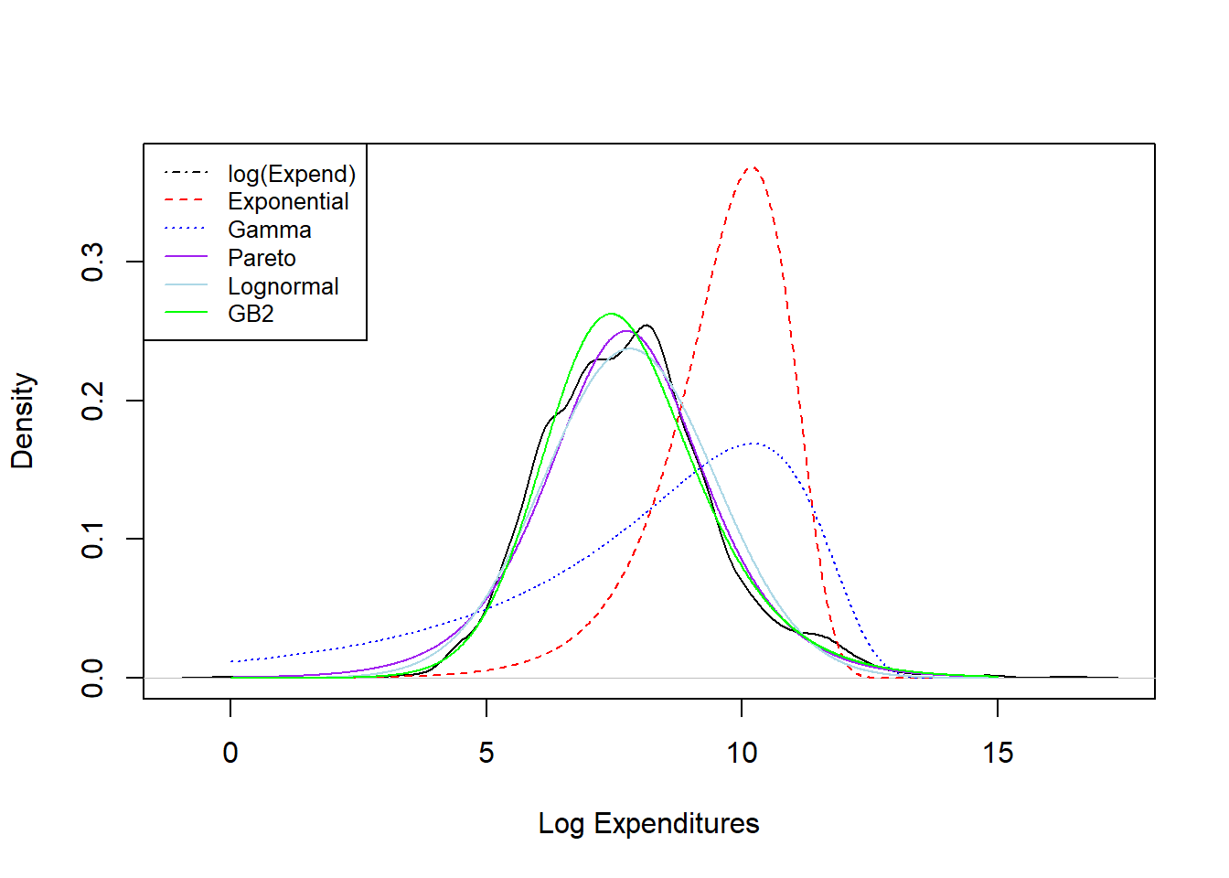
Figure 4.9: Density Comparisons for the Wisconsin Property Fund

Results from the fitting exercise are summarized in Figure 4.9. Here, the black “longdash” curve is a smoothed histogram of the actual data (that we will introduce in Section ??); the other curves are parametric curves where the parameters are computed via maximum likelihood. We see poor fits in the red dashed line from the exponential distribution fit and the blue dotted line from the gamma distribution fit. Fits of the other curves, Pareto, lognormal, and GB2, all seem to provide reasonably good fits to the actual data. Chapter 6 describes in more detail the principles of model selection.

---

4.4.2.4 Starting Values

Generally, maximum likelihood is the preferred technique for parameter estimation because it employs data more efficiently. (See Appendix Chapter 19 for precise definitions of efficiency.) However, methods of moments and percentile matching are useful because they are easier to interpret and therefore allow the actuary or analyst to explain procedures to others. Additionally, the numerical estimation procedure (e.g. if performed in R) for the maximum likelihood is iterative and requires starting values to begin the recursive process. Although many problems are robust to the choice of the starting values, for some complex situations it can be important to have a starting value that is close to the (unknown) optimal value. Method of moments and percentile matching can produce desirable estimates without a serious computational investment and can thus be used as a starting value for computing maximum likelihood.

Show Quiz Solution

---

4.5 Exercises with a Practical Focus

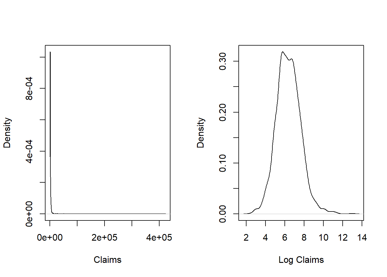
Exercise 4.1. Corporate Travel This exercise is based on the data set introduced in Exercise 1.1 where now the focus is on severity modeling. As in Exercise 3.14, we fit data for the period 2006-2021 but restrict claims to be greater than or equal to 10 (Australian dollars).

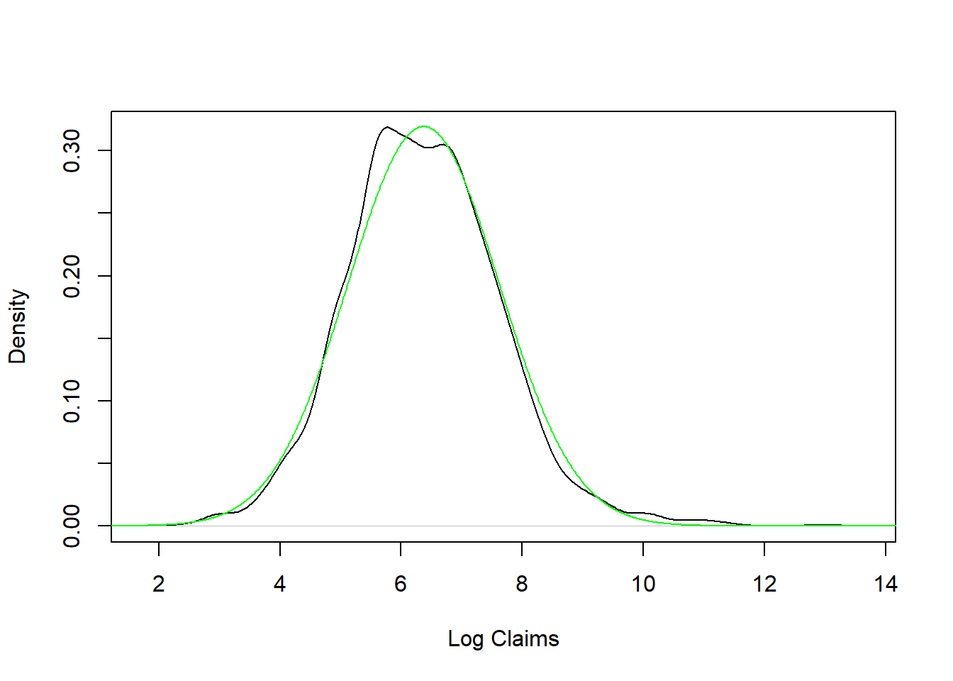
• a. Using the R function density, provide a nonparametric density estimate of the claims on both the original and logarithmic scale over the range of the data. Use this display to verify that the display is more interpretable on the logarithmic scale.
• b. Fit a normal distribution to logarithmic claims and compare the fitted distribution to the nonparametric (empirical) distribution. Interpret this comparison to mean that the lognormal distribution is an excellent candidate to represent these data.
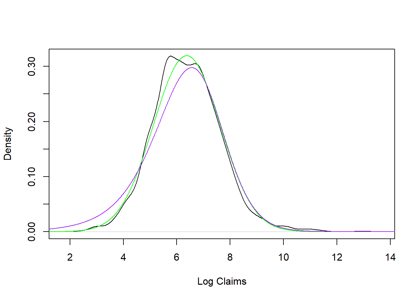
• c. As an alternative, fit a Pareto distribution to the claims data using maximum likelihood. To check your work, do this in two ways. A basic approach is to create a log likelihood function and minimize it (using the function optim). A second approach is to the the vglm function from the VGAM package.
• d. We have fit \(X\) to be a Pareto distribution but wish to plot \(Y=\ln(X)\). From Section 4.3.1.3, we saw that \(F_Y(y) = F_X(e^y)\) and \(f_Y(y) = e^y f_X(e^y)\). Use this transformation to augment the plot in part (b) to include the Pareto distribution.

From this analysis, you learn that the lognormal and Pareto distribution fit the data approximately the same with the lognormal as a slight favorite.

Solutions for Exercise 4.1

# Part a.
TravelClaims <- read.csv("Data\\ANUTravelClaims2022.csv", header = T)
TravelClaimsGT10 <- subset(TravelClaims, Incurred.Loss >= 10)
X <- TravelClaimsGT10$Incurred.Loss
par(mfrow = c(1, 2))
plot(density(X), main = "", xlab = "Claims")
plot(density(log(X)), main = "", xlab = "Log Claims")

# Part b.
y <- seq(0, 15, by = 0.01)
plot(density(log(X)), main = "", xlab = "Log Claims")
fit.norm <- dnorm(y, mean = mean(log(X)), sd = sd(log(X)))
lines(y, fit.norm, col = "green", lty = 7)

fit.norm <- dnorm(y, mean = mean(log(X)), sd = sd(log(X)))

# Part c.
library(VGAM)
# Pareto
fit.pareto <- vglm(X ~ 1, paretoII, loc = 0)
coef(fit.pareto)

(Intercept):1 (Intercept):2 
     7.275646      0.718753 

loglikPareto <- function(parms) {
    r <- parms[1]
    beta <- parms[2]
    nloglike <- -sum(log(VGAM::dparetoII(X, loc = 0, shape = exp(parms[2]), scale = exp(parms[1]))))
    return(nloglike)
}
Pareto.exp <- optim(par = c(1, 1), loglikPareto)
Pareto.exp$par

[1] 7.2751491 0.7187598

# Part d.
fpareto_ex <- VGAM::dparetoII(exp(y), loc = 0, shape = exp(coef(fit.pareto)[2]),
    scale = exp(coef(fit.pareto)[1])) * exp(y)
plot(density(log(X)), main = "", xlab = "Log Claims")
lines(y, fit.norm, col = "green", lty = 7)
lines(y, fpareto_ex, col = "purple", lty = 7)

Exercise 4.2. Wisconsin Property Fund. Replicate the real-data example introduced in Example 4.4.12 using the techniques demonstrated in Exercise 4.1.

Exercise 4.3. Group Personal Accident. This exercise is based on the data set introduced in Exercise 1.2. We use incurred claims for all available years, still omitting those less than 10.

One can fit a distribution to the losses. An analysis, summarized in Figure 4.10, shows the results from fitting via maximum likelihood the gamma, Pareto, and lognormal distributions to incurred losses. This figure suggests that the lognormal distribution appears to be the best fit.

Following the outlines in Exercises 4.1 and 4.2, fit these data via maximum likelihood and reproduce the figure that summarizes the results.

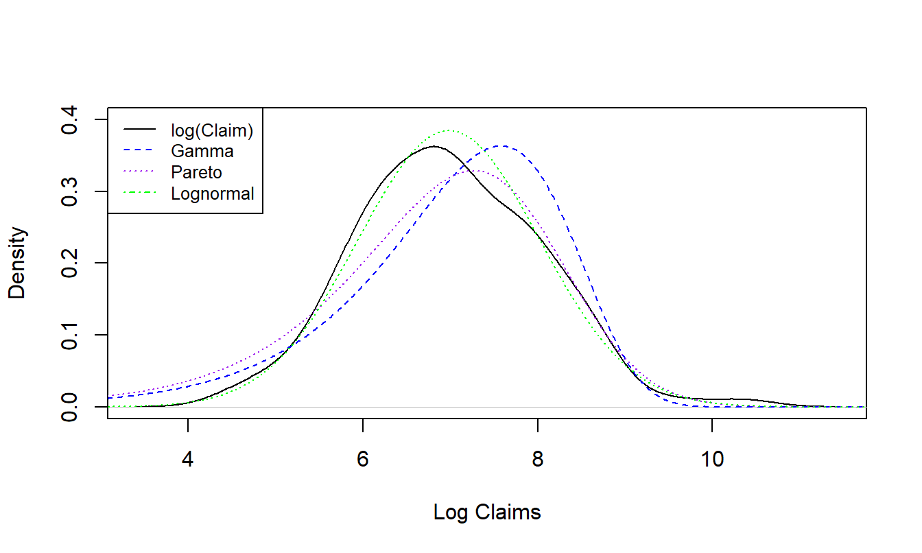
Figure 4.10: Distribution of Group Personal Accident Losses with Superimposed Fitted Distributions

Solutions for Exercise 4.3

GPAClaims <- read.csv("Data\\ANUGroupPersonalAccidentClaims2022.csv", header = T)
GPAClaimsGT10 <- subset(GPAClaims, Incurred.Loss >= 10)

library(VGAM)
x <- seq(0, 15, by = 0.01)

# Inference assuming a gamma distribution
fit.gamma <- vglm(Incurred.Loss ~ 1, family = gamma2, data = GPAClaimsGT10)
theta <- exp(coef(fit.gamma)[1])/exp(coef(fit.gamma)[2])  # theta = mu / alpha
alpha <- exp(coef(fit.gamma)[2])
fgamma_ex <- dgamma(exp(x), shape = alpha, scale = theta) * exp(x)

# Pareto
fit.pareto <- vglm(Incurred.Loss ~ 1, paretoII, loc = 0, data = GPAClaimsGT10)
fpareto_ex <- dparetoII(exp(x), loc = 0, shape = exp(coef(fit.pareto)[2]), scale = exp(coef(fit.pareto)[1])) *
    exp(x)

# Lognormal
fit.LN <- vglm(Incurred.Loss ~ 1, family = lognormal, data = GPAClaimsGT10)
flnorm_ex <- dlnorm(exp(x), mean = coef(fit.LN)[1], sd = exp(coef(fit.LN)[2])) *
    exp(x)

plot(density(log(GPAClaimsGT10$Incurred.Loss)), main = "", xlab = "Log Claims", ylim = c(0,
    0.4))

lines(x, fgamma_ex, col = "blue", lty = 2)
lines(x, fpareto_ex, col = "purple", lty = 3)
lines(x, flnorm_ex, col = "green", lty = 3)
legend("topleft", c("log(Claim)", "Gamma", "Pareto", "Lognormal"), cex = 0.8, lty = c(1,
    2, 3, 4, 1, 1), col = c("black", "blue", "purple", "green"))

4.6 Further Resources and Contributors

Contributors

• Zeinab Amin, The American University in Cairo, is the principal author of the initial version and also the second edition of this chapter. Email: zeinabha@aucegypt.edu for chapter comments and suggested improvements.
• Many helpful comments have been provided by Hirokazu (Iwahiro) Iwasawa, iwahiro@bb.mbn.or.jp .
• Other chapter reviewers include: Rob Erhardt, Samuel Kolins, Tatjana Miljkovic, Michelle Xia, and Jorge Yslas.

Further Readings and References

Notable contributions include: Cummins and Derrig (2012), Frees and Valdez (2008), Klugman, Panjer, and Willmot (2012), Kreer et al. (2015), McDonald (1984), McDonald and Xu (1995), Tevet (2016), and G. Venter (1983).

If you would like additional practice with R coding, please visit our companion LDA Short Course. In particular, see the Modeling Loss Severity Chapter.

Bibliography

Cummins, J. David, and Richard A. Derrig. 2012. Managing the Insolvency Risk of Insurance Companies: Proceedings of the Second International Conference on Insurance Solvency. Vol. 12. Springer Science & Business Media.

Frees, Edward W, and Emiliano A. Valdez. 2008. “Hierarchical Insurance Claims Modeling.” Journal of the American Statistical Association 103 (484): 1457–69.

Klugman, Stuart A., Harry H. Panjer, and Gordon E. Willmot. 2012. Loss Models: From Data to Decisions. John Wiley & Sons.

Kreer, Markus, Ayşe Kızılersü, Anthony W Thomas, and Alfredo D Egı́dio dos Reis. 2015. “Goodness-of-Fit Tests and Applications for Left-Truncated Weibull Distributions to Non-Life Insurance.” European Actuarial Journal 5 (1): 139–63.

McDonald, James B. 1984. “Some Generalized Functions for the Size Distribution of Income.” Econometrica: Journal of the Econometric Society, 647–63.

McDonald, James B, and Yexiao J Xu. 1995. “A Generalization of the Beta Distribution with Applications.” Journal of Econometrics 66 (1-2): 133–52.

Tevet, Dan. 2016. “Applying Generalized Linear Models to Insurance Data.” Predictive Modeling Applications in Actuarial Science: Volume 2, Case Studies in Insurance, 39.

Venter, Gary. 1983. “Transformed Beta and Gamma Distributions and Aggregate Losses.” In Proceedings of the Casualty Actuarial Society, 70:289–308. 133 & 134.