Chapter 15 Experience Rating using Bonus-Malus
Chapter Preview. This chapter introduces bonus-malus system used in motor insurance ratemaking. In particular, the chapter discusses the features of bonus-malus system and studies its modelling and properties via basic statistical techniques. Section 15.1 introduces the use of bonus-malus system as an experience rating scheme, followed by Section 15.2 which describes its practical implementation in several countries. Section 15.3 covers its modelling setup by a discrete time Markov Chain. Next, Section 15.4 studies a number of simple relevant properties associated with the stationary distribution of bonus-malus system. Section 15.5 focuses on the determination of a posteriori premium rating to complement a priori ratemaking.
15.1 Introduction
In this section, you learn how to:
- Use bonus-malus system as an experience rating scheme.
- Compare bonus-malus system with risk classification (Chapter 8) and credibility premium (Chapter 9).
Bonus-malus systemA type of rating mechanism where insured premiums are adjusted based on their individual loss experience history, which is used interchangeably as “no-fault discount,” “merit rating,” “experience rating” or “no-claim discount” in different countries, is based on penalizing insureds who are responsible for one or more claims by a premium surcharge (malus), and rewarding insureds with a premium discount (bonus) if they do not have any claims. Insurers use bonus-malus system (BMS) for two main purposes: to encourage drivers to drive more carefully in a policy year without any claims, and to ensure insureds to pay premiums proportional to their risks based on their claims experience via an experience rating mechanism.
BMS is an experience rating system commonly used in motor insurance. It represents an attempt to categorize insureds into homogeneous groups who pay premiums based on their claims experience. Depending on the rules in the scheme, new policyholders may be required to pay full premium initially, and obtain discounts in the future years as a result of claim-free years. BMS rewards policyholders for not making any claims during a policy year. In other words, it grants a bonus to a careful driver. This bonus principle may affect policy holders’ decisions whether to claim or not to claim, especially when involving accidents with slight damages, which is known as the ‘hunger for bonusPhenomenon where insureds under an experience rating system are dissuaded from filing minor claims in order to keep their no-claims discount’ phenomenon. The ‘hunger for bonus’ under a BMS may reduce insurers’ claim costs, and may be able to offset the expected decrease in premium income.
In motor insurance, BMS is a form of a posteriori rating to complement the use of a priori risk classification described in Chapter 11. The a priori risk classification divides portfolio of drivers into a number of homogeneous risk classes based on rating factors, such that policyholders in the same risk class pay the same premium. The ideal a posteriori mechanism is the credibility premium developed in Chapter 12, whereby premiums are derived on an individual basis for each policyholder by incorporating both the a priori and a posteriori information. However, such individual premium determination is overly complex from a commercial standpoint for practical implementations by motor insurers. For this reason, BMS is the preferred solution and it consists of three elements: bonus-malus classes, transition rules, and premium levels (also known as premium relativities). The advantage of using BMS is that the bonus-malus classes and the transition rules are pre-specified in advance by insurers. The bonus-malus classes and transition rules will be discussed in the next section.
15.2 BMS in Several Countries
In this section, you learn how to:
- Use BMS in Malaysia and other countries.
- Determine a transition rule.
Many countries around the world have adopted some form of BMS in their automobile insurance. The specifics of these systems can vary from country to country, but the general idea is to reward safe driving behavior by reducing premiums for policyholders who do not make claims, and increasing premiums for those who do. Some of the countries that have implemented or adopted the BMS are France, Germany, Italy, Spain and United Kingdom from Europe, and Malaysia, Hong Kong, Taiwan, Singapore and Korea from Asia. Please refer to Lemaire and Hongmin (1994), Lemaire (1998) and Park et. al (2010) for implementation of other BMS around the world.
15.2.1 BMS in Malaysia
Before the liberalization of Motor Tariff on 1st July 2017, the rating of motor insurance in Malaysia was governed by the Motor Tariff. Under the tariff, the rate charged should not be lower than the rates specified under the classes of risks. The basic risk classes considered were scope of insurance, cubic capacity of vehicle and estimated value of vehicle (or sum insured, whichever is lower). The final premium to be paid is adjusted by the policyholder’s claim experience, or equivalently, his bonus-malus entitlement.
Effective on 1st July 2017, the premium rates for motor insurance are liberalized, or de-tariffed. The pricing of premium is now determined by individual insurers and takafulCo-operative system of reimbursement or repayment in case of loss as an insurance alternative operators, and the consumers are able to enjoy a wider choice of motor insurance products at competitive prices. Since tariff liberalization encourages innovation and competition among insurers and takaful operators, the premiums are based on broader risk factors other than the risk classes specified in the Motor Tariff. Other rating factors may be defined in the risk profile of an insured, such as age of vehicle, age of driver, safety and security features of vehicle, geographical location of vehicle and traffic offences of driver. However, the bonus-malus entitlement from the Motor Tariff remains ‘unchanged’ and continue to exist, and is ‘transferable’ from one insurer, or from one takaful operator, to another.
The discounts in the Malaysian BMS are divided into six classes, starting from the initial class of 0% discount, followed by classes of 25%, 30%, 38.3%, 45% and 55% discounts. A claim-free policy year indicates that a policyholder is entitled to move one-step forward to the next discount class, such as from a 0% discount to a 25% discount in the renewal year. If a policyholder is already at the highest class, which is at a 55% discount, a claim-free policy year indicates that the policyholder remains in the same class. On the other hand, if one or more claims are made within the policy year, the discount will be forfeited and the policyholder has to start at 0% discount in the renewal year. This set of transition rules can also be summarized as a rule of -1/Top, that is, a class of bonus for a claim-free year, and moving to the highest class after having one or more claims. For an illustration purpose, Figure 15.1 shows the classes and the transition diagram for the Malaysian BMS.
| Classes | Discounts (%) |
|---|---|
| 0 | 0.00 |
| 1 | 25.00 |
| 2 | 30.00 |
| 3 | 38.33 |
| 4 | 45.00 |
| 5 (and above) | 55.00 |
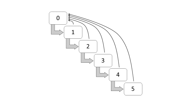
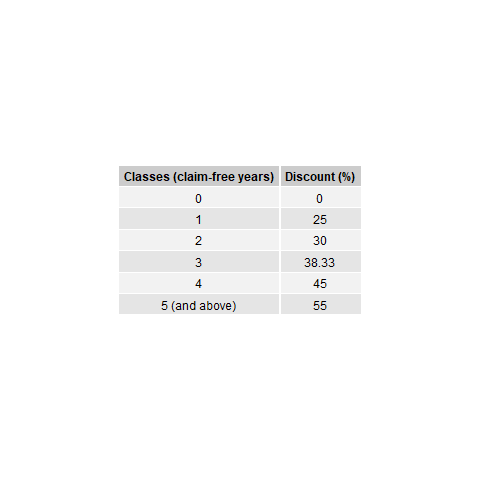
Figure 15.1: Transition diagram for bonus-malus classes (Malaysia)
15.2.2 BMS in Other Countries
The BMS in Brazil are subdivided into seven classes, with the following premium levels (Lemaire and Zi 1994): 100, 90, 85, 80, 75, 70, and 65. These premium levels are entitled to the following discounts: 0%, 10%, 15%, 20%, 25%, 30% and 35%. New policyholders have to start at 0% discount, or at premium level 100. A claim-free policy year indicates that a policyholder can move forward at a one-class discount. If one or more claims incurred within the policy year, the policyholder has to move one-class backward for each claim. Figure 15.2 shows the classes and the transition diagram for the BMS in Brazil. This set of transition rules can also be summarized as a rule of -1/+1, that is, a class of bonus for a claim-free policy year, and a class of malus for each claim reported.
| Classes | Discounts (%) |
|---|---|
| 0 | 0 |
| 1 | 10 |
| 2 | 15 |
| 3 | 20 |
| 4 | 25 |
| 5 | 30 |
| 6 (and above) | 35 |
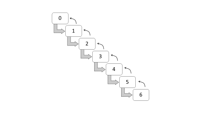
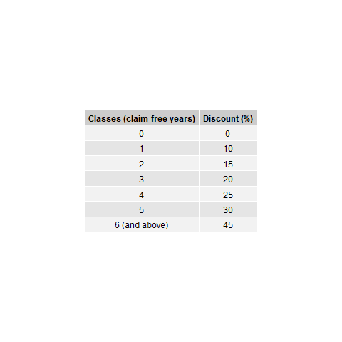
Figure 15.2: Transition diagram for bonus-malus classes (Brazil)
The BMS in Switzerland are subdivided into twenty-two classes, with the following premium levels: 270, 250, 230, 215, 200, 185, 170, 155, 140, 130, 120, 110, 100, 90, 80, 75, 70, 65, 60, 55, 50 and 45 (Lemaire and Zi 1994). The premium levels 270, 250, 230, 215, 200, 185, 170, 155, 140, 130, 120 and 110 are the premiums with the following loadings (malus): 170%, 150%, 130%, 115%, 100%, 85%, 70%, 55%, 40%, 30%, 20%, and 10%. On the other hand, the premium levels 100, 90, 80, 75, 70, 65, 60, 55, 50 and 45 are the premiums with the following discounts (bonus): 0%, 10%, 20%, 25%, 30%, 35%, 40%, 45%, 50% and 55%. New policyholders have to start at 0% discount, or at premium level 100, and a claim-free policy year indicates that a policyholder can move one-class forward. If one or more claims incurred within the policy year, the policyholder has to move four-classes backward for each claim. Table 15.1 and Figure 15.3 respectively show the classes and the transition diagram for the BMS in Switzerland. This set of transition rule can be summarized as a rule of -1/+4. It should be noted that the entry level is at class 12, which is at premium level 100 (or 0% discount).
Table 15.1 Bonus-malus classes (Switzerland)
\[ \small{ \begin{array}{*{20}c} \hline \text{Classes} & \text{Loadings } (\%) & \text{Classes} & \text{Discounts } (\%)\\ \hline {0} & {170} & {12} & {0}\\ {1} & {150} & {13} & {10}\\ {2} & {130} & {14} & {20}\\ {3} & {115} & {15} & {25}\\ {4} & {100} & {16} & {30}\\ {5} & {85} & {17} & {35}\\ {6} & {70} & {18} & {40}\\ {7} & {55} & {19} & {45}\\ {8} & {40} & {20} & {50}\\ {9} & {30} & {21} & {55}\\ {10} & {20} && \\ {11} & {10} && \\ \hline \end{array} } \]
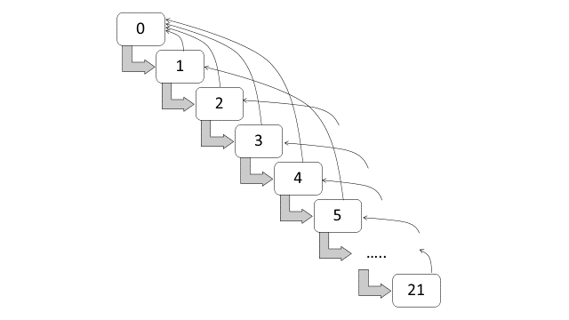
Figure 15.3: Transition diagram for bonus-malus classes (Switzerland)
15.3 BMS and Markov Chain Model
In this section, you learn how to:
- Represent bonus-malus classes using transition probabilities.
- Use yjr transition matrix.
A BMS can be represented by a discrete time Markov chainA stochastic model (time dependent) where the probability of each event depends only on the current state and not the historical path. A stochastic process is said to possess the Markov property if the evolution of the process in the future depends only on the present state but not the past. A discrete time Markov Chain is a Markov process with discrete state space.
15.3.1 Transition Probability
A Markov Chain is determined by its transition probabilities. The transition probability from state \(i\) (at time \(n\)) to state \(j\) (at time \(n + 1\)) is called a one-step transition probability, and is denoted by \(p_{ij}(n,n+1) = Pr (X_{n + 1} = j|X_n = i)\), \(i = 1,2,\ldots,k\), \(j = 1,2,\ldots,k\). For general transition from time \(m\) to time \(n\), for \(m<n\), by conditioning on \(X_{o}\) for \(m\le o\le n\), we have the Chapman-Kolmogorov equation of
\[ p_{ij}(m,n)=\sum_{l\in S} p_{il}(m,o)p_{lj}(o,n). \]
A time-homogeneous Markov Chain satisfies the property of \(p_{ij}(n,n+t)=p_{ij}^{(t)}\) for all \(n\). For instance, we have \(p_{ij}(n,n+1)=p_{ij}^{(1)}\equiv p_{ij}\). In this case, the Chapman-Kolmogorov equation can be written as
\[ p_{ij}(0,m+n)=\sum_{l\in S} p_{il}(0,m)p_{lj}(m,m+n)=\sum_{l\in S}p_{il}^{(m)}p_{lj}^{(n)}. \]
In the context of BMS, the transition of the bonus-malus classes is governed by the transition probability in a given policy year. The transition of the bonus-malus classes is also a time-homogeneous Markov Chain since the set of transition rules is fixed and independent of time. We can represent the one-step transition probabilities by a \(k \times k\) transition matrix \({\bf P}=(p_{ij})\) that corresponds to bonus-malus classes \(0,1,2,\ldots,k-1\).
\[ \small{ {\bf P} = \left[ {\begin{array}{*{20}c} p_{00} & p_{01} & \ldots & & & p_{0k-1} \\ p_{10} & p_{11} & \ldots & & & p_{1k-1} \\ \vdots & \ddots & & & & \vdots \\ p_{k-10} & p_{k-11} & \cdots & & & p_{k-1k-1} \end{array} } \right] } \]
Here, its \((i,j)\)-th element is the transition probability from state \(i\) to state \(j\). In other words, each row of the transition matrixMatrix that represents all probabilities for transition from one state to another (could be same state) for a markov chain represents the transition of flowing out of state, whereas each column represents the transition of flowing into the state. The summation of transition probabilities of flowing out of state must equal to 1, or each row of the matrix must sum to 1, i.e. \(\sum_j p_{ij} = 1\). All probabilities must be non-negative, i.e. \(p_{ij} \ge 0\).
15.3.2 Some Applications
Consider the Malaysian BMS. Let \(\{X_{t}:t=0,1,2,\ldots\}\) be the bonus-malus class occupied by a policyholder at time \(t\) with state space \(S=\{0,1,2,3,4,5\}\). Therefore, the transition probability in a no-claim policy year is equal to the probability of transition from state \(i\) to state \(i+1\), i.e. \(p_{ii+1}\). If an insured has one or more claims within the policy year, the probability of transitioning back to state 0 is represented by \(p_{i0}=1-p_{ii+1}\). Hence, the Malaysian BMS can be represented by the following \(6\times 6\) transition matrix:
\[ \small{ {\bf P} = \left[ {\begin{array}{*{20}c} p_{00}&p_{01}&0&0&0&0\\ p_{10}&0&p_{12}&0&0&0\\ p_{20}&0&0&p_{23}&0&0\\ p_{30}&0&0&0&p_{34}&0\\ p_{40}&0&0&0&0&p_{45}\\ p_{50}&0&0&0&0&p_{55} \end{array} }\right] = \left[ {\begin{array}{*{20}c} {1 - p_{01}}&p_{01}&0&0&0&0\\ {1 - p_{12}}&0&p_{12}&0&0&0\\ {1 - p_{23}}&0&0&p_{23}&0&0\\ {1 - p_{34}}&0&0&0&p_{34}&0\\ {1 - p_{45}}&0&0&0&0&p_{45}\\ {1 - p_{55}}&0&0&0&0&p_{55} \end{array} }\right] } \]
Example 15.3.1. Provide the transition matrix for the BMS in Brazil.
Show Example Solution
Example 15.3.2. Provide the transition matrix for the BMS in Switzerland.
Show Example Solution
15.4 BMS and Stationary Distribution
In this section, you learn how to:
- Calculate stationary probabilities.
- Observe a premium evolution.
- Measure the convergence rate.
15.4.1 Stationary Distribution
A stationary probability, which is also known as a steady-state probability, is a probability of being in a state at equilibrium or in the long run. In a Markov chain, each state has a corresponding stationary probability. These probabilities do not change over time once the Markov chain has achieved its steady state. Stationary probability is important for understanding the long-term behavior, equilibrium states, and predictive aspects of a system (such as BMS) which are modeled using a Markov chain. In this section, we introduce a stationary probability because it offers some practical applications of the BMS.
Stationary probabilities can be represented by a row vector \(\boldsymbol \pi =(\pi_{1},\pi_{2},\ldots,\pi_{k})\) with the following properties:
\[ \begin{align}0\le \pi_{j}\le 1,\notag\\\sum\limits_{j}\pi_{j}=1,\notag\\\pi_{j}=\sum\limits_{i}\pi_{i}p_{ij}.\end{align} \]
The last equation can be written in terms of matrix and vector, which is \(\boldsymbol\pi \bf P=\boldsymbol\pi\), where \(\boldsymbol\pi\) is the stationary probability vector and \(\bf P\) is the transition matrix. The first two conditions are necessary for the probability distribution, whereas the last property indicates that \(\boldsymbol\pi\) is invariant (i.e. unchanged) by the one-step transition matrix. In other words, once the Markov Chain has reached stationary state, its probability distribution will stay stationary over time. Mathematically, the stationary vector \(\boldsymbol\pi\) can also be obtained by finding the left eigenvector of the one-step transition matrix.
Example 15.4.1. Find the stationary distribution for the BMS in Malaysia assuming that the probability of a no-claim policy year for all bonus-malus classes are equal, and it is equivalent to \({p_0}\).
Show Example Solution
The stationary distribution shown in Example 15.4.1 represents the asymptotic distribution of the BMS, or the distribution in the long run. As an example, assuming that the probability of a no-claim policy year is \(p_0 = 0.90,\) the stationary probabilities are:
\[ \small{ \begin{array}{l} {\pi _0} = 1 - {p_0} = 0.1000\\ {\pi _1} = (1 - {p_0}){p_0} = 0.0900\\ {\pi _2} = (1 - {p_0}){p_0}^2 = 0.0810\\ {\pi _3} = (1 - {p_0}){p_0}^3 = 0.0729\\ {\pi _4} = (1 - {p_0}){p_0}^4 = 0.0656\\ {\pi _5} = {p_0}^5 = 0.5905 \end{array} } \]
In other words, \({\pi_0} = 0.10\) indicates that 10% of insureds will eventually belong to class 0, \({\pi _1} = 0.09\) indicates that 9% of insureds will eventually belong to class 1, and so forth, until \({\pi _5} = 0.59\), which indicates that 59% of insureds will eventually belong to class 5.
15.4.2 R Code for a Stationary Distribution
We can use the left eigenvector of a transition matrix to calculate a stationary distribution. The following R code can be used to calculate a stationary distribution in two stages:
- Create a Transition Matrix
- Find a stationary distribution using left eigenvector.
Show the R Code for a Stationary Distribution
Example 15.4.2. Consider the BMS in Brazil where the transition rule is -1/+1. Let the probability of a no-claim policy year (probability of one-class forward) equal to \(p_0\), the probability of one or more claims in a policy year (probability of one-class backward) equal to \(p_1\), the probability of one or more claims in the next policy year (probability of two-classes backward) equal to \(p_2\), and so on and so forth. Find the stationary distribution assuming that \(p_k\) is distributed as Poisson with probability
\[ p_k = \frac{e^{ - 0.1}{(0.1)}^k}{{k!}},{\rm{ }}k = 0,1,2,\ldots \]
Show Example Solution
Example 15.4.3. Using the results from Example 15.4.2, find the mean premium under the steady state condition assuming that the premium prior to implementing the bonus-malus discount is 1000.
Show Example Solution
The results indicate that the final premium reduce from 1000 to 656.5 in the long run under stationary condition if the discount is considered. From a financial standpoint, this implies that the collected premium is insufficient to cover the expected claim cost of 1000. This result is not surprising because none of the BMS classes in Brazil impose a malus loading for the policyholders. More importantly, it indicates that the BMS will only be financially balanced if there are both bonus and malus classes and the premium levels are re-calculated such that the expected premium under the stationary distribution equals to 1000.
15.4.4 R Code for Premium Evolution
The following R code can be used to find the premium in the n-th year and the premiums in 20 years under the BMS in Malaysia (to find the solution in Example 15.4.4). A function for transition matrix is created so that it can be used in the later sections (Section 15.5).
- Create a function for transition matrix
- Create a function for the n-th power of a square matrix
- Create a function for premium in n-th year
- Provide premiums for 20 years,
Show the R Code for Premium Evolution
Example 15.4.5. Using the results from Example 15.4.2, observe the mean premiums in 20 years under the BMS in Brazil, assuming that the premium prior to implementing the bonus-malus discount is 1000.
Show Example Solution
The results in Examples 15.4.4-15.4.5 allow us to observe the evolution of mean premium for the BMS in Malaysia and Brazil. The evolution of premiums for both countries are provided in Table 15.4, and are shown graphically in Figure 15.4.
Table 15.4 Evolution of Premium (Malaysia and Brazil)
\[ \small{ \begin{array}{ccc|ccc} \hline \text{Year} & \text{Premium} & \text{Premium} & \text{Year} & \text{Premium} & \text{Premium} \\ & \text{Malaysia} & \text{Brazil} & & \text{Malaysia} & \text{Brazil} \\ \hline 1 & 625.5 & 766.9 & 11 & 565.8 & 657.2 \\ 2 & 598.7 & 737.6 & 12 & 565.8 & 656.9 \\ 3 & 580.6 & 713.1 & 13 & 565.8 & 656.7 \\ 4 & 570.6 & 693.8 & 14 & 565.8 & 656.6 \\ 5 & 565.8 & 679.2 & 15 & 565.8 & 656.6 \\ 6 & 565.8 & 669.3 & 16 & 565.8 & 656.6 \\ 7 & 565.8 & 664.0 & 17 & 565.8 & 656.6 \\ 8 & 565.8 & 660.5 & 18 & 565.8 & 656.5 \\ 9 & 565.8 & 658.8 & 19 & 565.8 & 656.5 \\ 10 & 565.8 & 657.7 & 20 & 565.8 & 656.5 \\ \hline \end{array} } \]
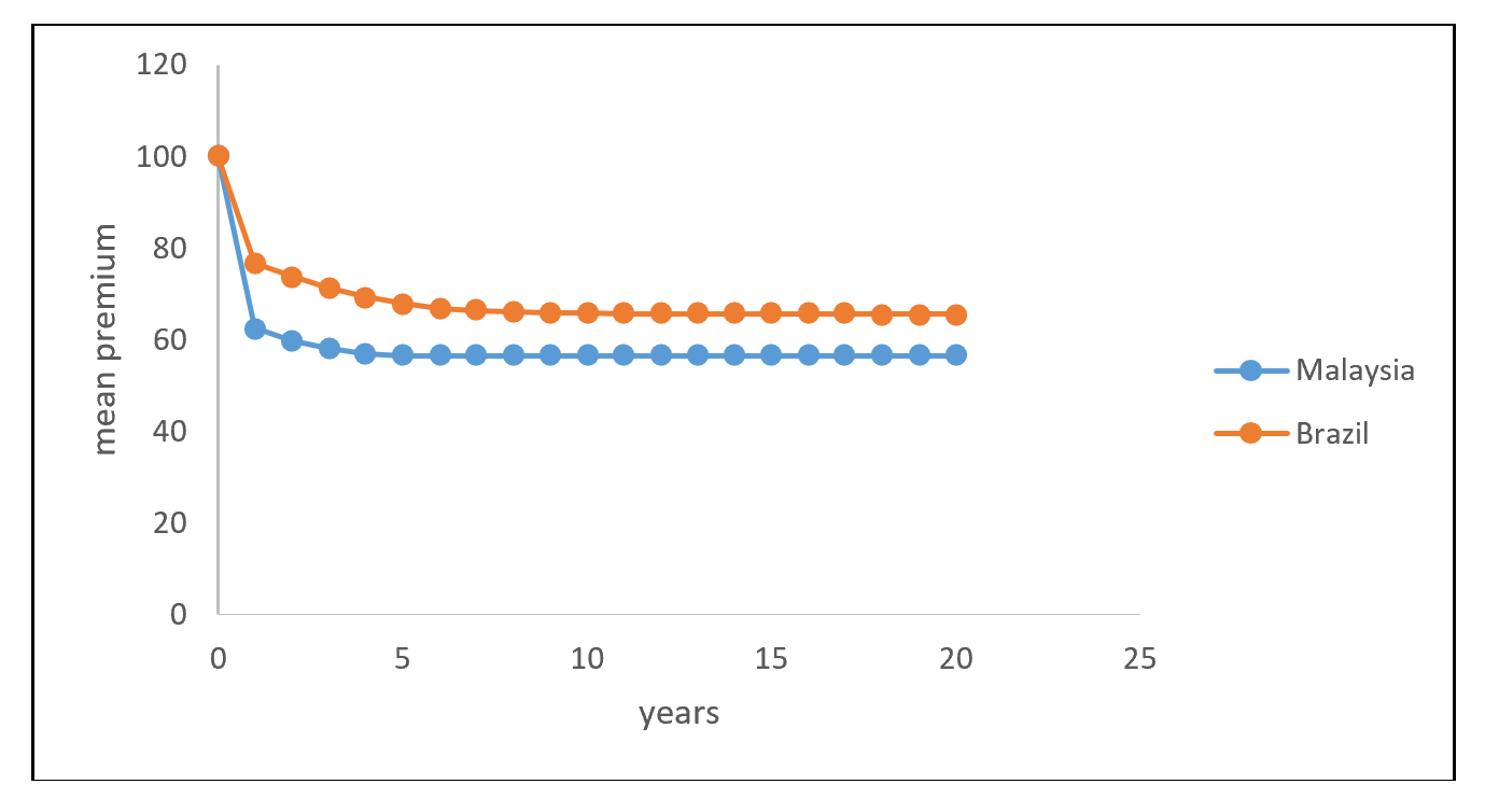
Figure 15.4: Evolution of Premium (Malaysia and Brazil)
The following R code can be used to create a function for the transition matrix under the BMS in Brazil. The function can be used to find the mean premium in the n-th year and the mean premiums in 20 years. The function can also be used in the later section (Section 15.5).
Show the R Code for Evolution of Premium (Malaysia and Brazil)
15.4.5 Convergence Rate
We may also be interested to determine the variation between the probability in the n-th year, \(p_{ij}^{(n)}\), and the stationary probability, \(\pi _j\). The variation between the probabilities can be measured using:
\[ \left| {average(p_{ij}^{(n)}) - {\pi _j}} \right|. \]
Therefore, the total variation can be measured by the sum of variation in all classes:
\[ \sum\limits_j\left| {average(p_{ij}^{(n)}) - {\pi _j}} \right|. \]
The total variation is also called the convergence rateAfter n transitions, the sum of variation between the probability in each state vs. the stationary probability because it measures the convergence rate after \(n\) years (or \(n\) transitions). A lower total variation implies a better convergence rate between the \(n\)-step transition probabilities and the stationary distribution.
Example 15.4.6. Using the results from Example 15.4.4, provide the total variations (convergence rate) in 20 years under the BMS in Malaysia.
Show Example Solution
15.4.6 R Code for Convergence Rate
The following R code can be used to calculate the total variation in the \(n\)th year, and the total variations (convergence rates) in 20 years under the BMS in Malaysia (the solution in Example 15.4.6).
- Recall the Transition Matrix
- Create a function for stationary probabilities
- Create a function for total variation in** **the n-th year
- Provide total variations (convergence rate) in 20 years
Show the R Code for Convergence Rate
Example 15.4.7. Provide the total variations (or convergence rate) in 20 years under the BMS in Brazil using the results from example 15.4.5.
Show Example Solution
Examples 15.4.6-15.4.7 provide the degree of convergence for two different BMS (two different countries). The Malaysian BMS reaches full stationary only after five years, while the BMS in Brazil takes a longer period. As mentioned in Lemaire (1998), a more sophisticated BMS would converge more slowly, and is considered as a drawback as it takes a longer period to stabilize. The main objective of a BMS is to separate the good drivers from the bad drivers, and thus, it is desirable to have a classification process that can be finalized (or stabilized) as soon as possible.
15.5 BMS and Premium Rating
In this section, you learn how to:
- Integrate priori information into optimal relativities.
- Calculate probability of staying in BMS level.
- Calculate constrained optimal relativities.
- Calculate unconstrained optimal relativities.
15.5.2 A Priori Risk Classification
Let us consider a portfolio of \(n\) policies, where the risk exposure (see Section 10.4) of driver \(i\) is denoted as \(m_{i}\) and the number of claims reported is represented by \(Y_{i}\), following from the notations used in Section 11.2. Let \({\bf x}_{i}^{T}=(x_{i1},x_{i2},\ldots, x_{iq})\) be the vector of observable variables for \(i=1,2,\ldots, n\). The Poisson regression as developed in Section 11.2 is commonly chosen to model \(Y_{i}\) under the generalized linear models (GLM) framework, see Section 13.3.2.2 and also McCullagh and Nelder (1989).
We can then express the predicted a priori expected claim frequency for policyholder \(i\) as
\[ \mu_{i}=m_{i}\lambda_{i}=m_{i}\exp\left(\hat{\beta}_{0}+\sum\limits_{m=1}^{q}\hat{\beta}_{m}x_{im}\right) , \]
where \(\hat{\beta}_{0},\hat{\beta}_{1},\ldots,\hat{\beta}_{q}\) are the estimated regression coefficients. In other words, \(\lambda_{i}=\frac{\mu_{i}}{m_{i}}\) is the expected claim frequency per unit exposure, which is the main focus of the a priori risk classification.
15.5.3 Modelling of Residual Heterogeneity
Since unobserved factors that may affect driving behaviors are not taken into account in estimating the expected claim frequency, insurers would have to account for the residual heterogeneity within each a priori risk class by introducing a random effect component \(\Theta_{i}\) into the conditional distribution of \(Y_{i}\). Given \(\Theta_{i}=\theta\), \(Y_{i}\) follows a Poisson distribution with mean \(\lambda_{i}\theta\), that is,
\[ \Pr(Y_{i}=k|\Theta_{i}=\theta)=\exp(-\lambda_{i}\theta)\frac{(\lambda_{i}\theta)^{k}}{k!},k=0,1,2,... \]
Following from the setup of gamma-Poisson model in Section 12.3.2, we further assume that all the \(\Theta_{i}\)’s are independent and follow a gamma \((a,a)\) distribution with the following density function as introduced in Appendix 20.2
\[ f(\theta)=\frac{1}{\Gamma(a)}a^{a}\theta^{a-1}\exp(-a\theta), \quad \theta > 0, \]
where the use of gamma-Poisson mixture produces a negative binomial distribution for \(Y_{i}\) (see Section 3.6). With these specifications, we obtain \(\mathrm{E}(\Theta_{i})=1\) and hence \(\mathrm{E}(Y_{i})=\mathrm{E}(\mathrm{E}(Y_{i}|\Theta_{i}))\) \(=\mathrm{E}(\lambda_{i}\Theta_{i})=\lambda_{i}\). by the law of iterated expectation in Appendix 18.2.1.
Furthermore, it can be shown that the posterior distribution of \(\Theta| y_{1}=k_{1},y_{2}=k_{2},\ldots,y_{n}=k_{n}\) is gamma distributed with parameters \(a+\sum_{j=1}^{n} k_{j}\) and \(a+n\lambda_{i}\) and therefore the Bayesian premium is given as
\[ \mathrm{E}(\lambda_{i}\Theta| y_{1}=k_{1},\ldots,y_{n}=k_{n})=\lambda_{i}\times\frac{a+\sum_{j=1}^{n} k_{j}}{a+n\lambda_{i}}. \]
On the other hand, applying the Bühlmann credibility-weighted estimate in Section 12.2 to the gamma-Poisson model in Section 12.3.2, we obtain
\[ \begin{array}{cl} EPV &=\mathrm{E}(\mathrm{Var}(Y|\lambda_{i}))=\mathrm{E}(\lambda_{i}\Theta)=\lambda_{i}, \\ VHM & =\mathrm{Var}(\mathrm{E}(Y|\lambda_{i}))=\mathrm{Var}(\lambda_{i}\Theta)=\frac{\lambda_{i}^{2}}{a},\\ K & =\frac{EPV}{VHM}=\frac{\lambda_{i}}{\frac{\lambda_{i}^{2}}{a}}=\frac{a}{\lambda_{i}},\\ Z & =\frac{n}{n+K}=\frac{n\lambda_{i}}{n\lambda_{i}+a},\\ \bar{Y} & =\frac{\sum_{j=1}^{n}y_{j}}{n}=\frac{\sum_{j=1}^{n}k_{j}}{n}, \\ \mu & =\mathrm{E}(\mathrm{E}(Y_{i}|\lambda_{i}))=\mathrm{E}(\lambda_{i}\Theta)=\lambda_{i}, \end{array} \]
and hence the credibility-weighted estimate as
\[ \begin{array}{cl} \mathrm{E}[\mathrm{E}(Y|\lambda_{i})|y_{1}=k_{1},...,y_{n}=k_{n}] & =\mathrm{E}[\lambda_{i}\Theta|y_{i}=k_{1},...,y_{n}=k_{n}] \\ & = Z\bar{Y}+(1-Z)\mu \\ & = \frac{n\lambda_{i}}{n\lambda_{i}+a}\frac{\sum_{j=1}^{n}k_{j}}{n}+\frac{a}{n\lambda_{i}+a}\lambda_{i} \\ & =\frac{\lambda_{i}(a+\sum_{j=1}^{n}k_{j})}{a+n\lambda_{i}} \end{array} \]
that is, the Bühlmann credibility premium exactly matches the Bayesian premium.
Despite the fact that the credibility premium derived on an individual basis above is the ideal a posteriori premium, in practice insurers make use of BMS as a discrete approximation to the Bayesian premium, due to the relatively simpler structure of BMS as compared to the individual calculations of credibility premium.
15.5.4 Stationary Distribution Allowing for Residual Heterogeneity
Suppose that a driver is selected at random from the portfolio that has been classified into \(h\) risk classes via the use of observed a priori variables. The true expected claim frequency for this driver is given by \(\Lambda\Theta\), where \(\Lambda\) is the unknown a priori expected claim frequency and \(\Theta\) is the random residual heterogeneity. Let us further denote \(w_{g}\) as the proportion of drivers in the \(g\)-th risk class, that is, \(w_{g}=\Pr(\Lambda=\lambda_{g})=\frac{n_{g}}{n}\) where \(n_{g}\) is the number of drivers classified in the \(g\)-th risk class. Note that since there are two different concepts of risk classes (from a priori risk classification) and BMS (or NCD) classes (for a posteriori rating mechanism), for the rest of this chapter we will refer BMS classes as BMS levels instead to avoid unnecessary confusion.
Let \(p_{ij}^{\lambda}(\lambda\theta)\) be the transition probability of moving from BMS level \(i\) to level \(j\) for a driver with expected claim frequency \(\lambda\theta\) belonging to the risk class with predicted claim frequency of \(\lambda\). In other words, the one-step transition matrix can be written as \({\bf P}(\lambda\theta; \lambda)=\{p_{ij}^{\lambda}(\lambda\theta)\}\). The row vector of the stationary distribution \(\boldsymbol \pi=(\pi_{0}^{\lambda}(\lambda\theta),\pi_{1}^{\lambda}(\lambda\theta),\ldots,\pi_{k-1}^{\lambda}(\lambda\theta))\) can be obtained by solving the following conditions:
\[ \begin{array}{cl} \boldsymbol\pi(\lambda\theta;\lambda)\bf P(\lambda\theta;\lambda) &=\boldsymbol\pi(\lambda\theta;\lambda) \\ \boldsymbol\pi(\lambda\theta;\lambda)\bf 1& =1 \end{array} \]
where \(\bf 1\) is the column vector of \(1\)’s and \(\pi_{\ell}^{\lambda}(\lambda\theta)\) is the stationary probability for a driver with true expected claim frequency of \(\lambda\theta\) to be in level \(\ell\) when the equilibrium steady state is reached in the long run.
Note that the equation for stationary distribution that allows for residual heterogeneity in this section, \(\boldsymbol\pi(\lambda\theta)\bf P(\lambda\theta)=\boldsymbol\pi(\lambda\theta)\) , is similar to the equation of stationary distribution in Section 15.4.1 where \(\boldsymbol\pi\bf P=\boldsymbol\pi\) . The only difference is that the stationary distribution \(\boldsymbol\pi(\lambda\theta)\) and the transition matrix \(\boldsymbol P(\lambda\theta)\) are written in terms of a function of \(\boldsymbol\lambda\theta\) .
With these setup, the probability of drivers staying in BMS level \(L=\ell\) for \(\ell=0,1,\ldots,k-1\) in the context of the entire portfolio can be obtained as
\[ \begin{array}{ll} \Pr(L=\ell) &=\sum\limits_{g=1}^{h}\Pr(L=\ell|\Lambda=\lambda_{g})\Pr(\Lambda=\lambda_{g}) \\ &=\sum\limits_{g=1}^{h}\Pr(\Lambda=\lambda_{g})\int_{0}^{\infty}\Pr(L=\ell|\Lambda=\lambda_{g},\Theta=\theta)f(\theta)d\theta \\ &=\sum\limits_{g=1}^{h}w_{g}\int_{0}^{\infty}\pi_{\ell}^{\lambda_{g}}(\lambda_{g}\theta)f(\theta)d\theta. \end{array} \]
From previous section (section 15.5.3), \(\Theta_{i}\) is the random effect component. As an example, if we assume that all \(\Theta_{i}\)’s are independent and follow a gamma \((a,a)\) distribution, then\(\ f(\theta)\) is the density function of a gamma \((a,a)\) distribution.
For further understanding, we provide R program to calculate the probability of staying in level \(L=\ell\), \(\Pr(L=\ell)\), for the Malaysian BMS. From previous sections, the functions for transition matrix and stationary distribution are functions of \(\lambda\). Therefore, the functions allow us to write R program to calculate \(\Pr(L=\ell)\). Similar R programs can be developed for the Brazilian BMS.
Example 15.5.1. Consider the BMS levels and the transition rules of the Malaysian system (-1/Top). Assume that the following 3 values of a priori expected claim frequency are given; \(\lambda_{1}=0.1\), \(\lambda_{2}=0.3\), \(\lambda_{3}=0.5\), with the following proportions (weights); \(\Pr(\Lambda=\lambda_{1})=0.6\), \(\Pr(\Lambda=\lambda_{2})=0.3\), \(\Pr(\Lambda=\lambda_{3})=0.1\). We also assume that the gamma parameter is fixed at \(a=1.5\). Calculate the probability of staying in level \(L=\ell\), \(\Pr(L=\ell)\).
Show Example Solution
The results indicate that in the long run and under residual heterogeneity, 16% of insureds will eventually belong to level \(\ell=\) 0, 11% of insureds will eventually belong to level \(\ell=1\), and so forth. The majority of insureds (more than half, i.e. 52%) will eventually occupy the highest level which is level \(\ell=5\).
15.5.5 Determination of Optimal Relativities
The optimal relativity for each BMS level was first derived by Norberg (1976) through the minimization of the following objective function, which is more commonly known as the Norberg’s criterion:
\[ \min\mathrm{E}((\bar{\lambda}\Theta-\bar{\lambda}r_{L})^2)=\min\mathrm{E}((\Theta-r_{L})^2), \]
where \(\bar{\lambda}\) is the constant expected claim frequency for all policyholders in the absence of a priori risk classification and \(r_{L}\) is the premium relativity for BMS level \(L\). It should be noted that when there is no risk classification, all \(\lambda\)’s are equal and they are represented by a constant \(\bar{\lambda}\).
Pitrebois, Denuit, and Walhin (2003) then incorporated the information of a priori risk classification into the optimization of the same objective function of
\[ \min\mathrm{E}((\Theta-r_{L})^2) \]
to derive \(r_{L}\) analytically. Tan et al. (2015) further proposed the minimization of the following objective function
\[ \min\mathrm{E}((\Lambda\Theta-\Lambda r_{L})^2),\text{ subject to }\mathrm{E}(r_{L})=1 \]
under a financial balanced constraint (that is, the expected premium relativity equals 1) to determine the optimal relativities of a BMS given pre-specified BMS levels and transition rules, where
\[ \begin{array}{ll} \min\mathrm{\mathrm{E}[(\Lambda\Theta-\Lambda r_{L})^2]} &=\sum\limits_{\ell=0}^{k-1}\mathrm{E}[(\Lambda\Theta-\Lambda r_{L})^2|L=\ell]\Pr(L=\ell) \\ &=\sum\limits_{\ell=0}^{k-1}\mathrm{E}(\mathrm{E}[(\Lambda\Theta-\Lambda r_{L})^2|L=\ell,\Lambda)|L=\ell]\Pr(L=\ell) \\ &=\sum\limits_{\ell=0}^{k-1}\sum\limits_{g-1}^{h}\mathrm{E}((\Lambda\Theta-\Lambda r_{L})^2|L=\ell,\Lambda=\lambda_{g})\Pr(\Lambda=\lambda_{g}|L=\ell)\Pr(L=\ell) \\ &=\sum\limits_{\ell=0}^{k-1}\sum\limits_{g=1}^{h}\int_{0}^{\infty}(\lambda_{g}\theta-\lambda_{g} r_{\ell})^2\pi_{\ell}(\lambda_{g}\theta)w_{g}f(\theta)d\theta \\ &=\sum\limits_{g=1}^{h}w_{g}\int_{0}^{\infty}\sum\limits_{\ell=0}^{k-1}(\lambda_{g}\theta-\lambda_{g}r_{\ell})^2\pi_{\ell}(\lambda_{g}\theta)f(\theta)d\theta. \end{array} \]
It is crucially important that the optimal relativity has an average of 100%, so that the bonuses and maluses exactly offset each other to result in a financial equilibrium condition. Note that the approach considered by Pitrebois, Denuit, and Walhin (2003) does not require the financial balanced constraint because the analytical solution to its objective function is given by \(r_{\ell}=\mathrm{E}(\Theta|L=\ell)\), so it follows that \(\mathrm{E}(r_{L})=\mathrm{E}\left(\mathrm{E}(\Theta|L)\right)=\mathrm{E}(\Theta)=1\) with the specific choice of gamma \((a,a)\) distribution for the random effect component \(\Theta\).
In this case, the optimization problem can be solved by specifying the Lagrangian as
\[ \begin{array}{ll} \mathcal{L}({\bf r},\alpha) &=\mathrm{E}((\Lambda\Theta-\Lambda r_{L})^2)+\alpha(\mathrm{E}(r_{L})-1) \\ &=\sum\limits_{\ell=0}^{k-1}\mathrm{E}((\Lambda\Theta-\Lambda r_{L})^2|L=\ell)\Pr(L=\ell)+\alpha(\sum\limits_{\ell=0}^{k-1}r_{\ell}\Pr(L=\ell)-1), \end{array} \]
where \({\bf r}=(r_{0},r_{1},\ldots,r_{k-1})^{T}\). The required first order conditions are given as follows
\[ \begin{array}{cl} \Pr(L=\ell)(2\mathrm{E}(\Lambda^2\Theta-\Lambda^2 r_{L}|L=\ell)-\alpha)&=0,\qquad \ell=0,1,...,k-1 \\ \sum\limits_{\ell=0}^{k-1}r_{\ell}\Pr(L=\ell)-1&=0. \end{array} \]
Finally, the solution set for \(\alpha\) and \(r_{\ell}, \ell=0,1,\ldots,k-1\) is obtained as
\[ \begin{array}{cl} \alpha &=\frac{(\sum\limits_{\ell=0}^{k-1}\frac{\mathrm{E}(\Lambda^2\Theta|L=\ell)}{\mathrm{E}(\Lambda^2|L=\ell)})-1}{\sum\limits_{\ell=0}^{k-1}\frac{\Pr(L=\ell)}{2\mathrm{E}(\Lambda^2|L=\ell)}}, \\ r_{\ell}&=\frac{\mathrm{E}(\Lambda^2\Theta|L=\ell)}{\mathrm{E}(\Lambda^2|L=\ell)}-\frac{\alpha}{2\mathrm{E}(\Lambda^2|L=\ell)}, \end{array} \]
where
\[ \begin{array}{cl} \Pr(L=\ell)&=\sum\limits_{g=1}^{h}w_{g}\int_{0}^{\infty}\pi_{\ell}^{\lambda_{g}}(\lambda_{g}\theta)f(\theta)d\theta, \\ \mathrm{E}(\Lambda^2\Theta|L=\ell)&=\frac{\sum\limits_{g=1}^{h}w_{g}\int_{0}^{\infty}\lambda_{g}^{2}\theta\pi_{\ell}^{\lambda_{g}}(\lambda_{g}\theta)f(\theta)d\theta}{\sum\limits_{g=1}^{h}w_{g}\int_{0}^{\infty}\pi_{\ell}^{\lambda_{g}}(\lambda_{g}\theta)f(\theta)d\theta}, \\ \mathrm{E}(\Lambda^2|L=\ell)&=\frac{\sum\limits_{g=1}^{h}w_{g}\int_{0}^{\infty}\lambda_{g}^{2}\pi_{\ell}^{\lambda_{g}}(\lambda_{g}\theta)f(\theta)d\theta}{\sum\limits_{g=1}^{h}w_{g}\int_{0}^{\infty}\pi_{\ell}^{\lambda_{g}}(\lambda_{g}\theta)f(\theta)d\theta}. \\ \end{array} \]
If we perform the optimization without the financial balanced constraint, then we obtain
\(\alpha^{\text{unconstrained}}=0,\) and \(r_{\ell}^{\text{unconstrained}}=\frac{\mathrm{E}(\Lambda^2\Theta|L=\ell)}{\mathrm{E}(\Lambda^2|L=\ell)}.\)
It should be noted that the optimal relativity \(r_{\ell}\) of each level \(\ell\) is the scale that determines the premium’s discount/loading to the insureds. If \(r_{\ell}<1\), then the insured receives a discount based on his favorable past performance. If \(r_{\ell}>1,\) then the insured is penalized and has to pay additional loading based on his past performance. The concept is similar to the discount under the BMS in Malaysia and Brazil which were discussed in previous sections. The difference is that the discounts under the BMS in Malaysia and Brazil were pre-determined (\(r_{\ell}\) =100%, 75%, 70%, 61.67%, 55%, 45% respectively for \(\ell\) =0,1,2,3,4,5 for BMS in Malaysia; \(r_{\ell}\) =100%, 90%, 85%, 80%, 75%, 70%, 65% respectively for \(\ell\) =0,1,2,3,4,5,6 for BMS in Brazil), whereas the relativities \(r_{\ell}\) under heterogeneous residual are determined using optimization (minimization of an objective function which is subjected to a constraint).
For further understanding, we provide R program to calculate the optimal relativity \(r_{\ell}\) under unconstrained method which allows for residual heterogeneity for the Malaysian BMS. From previous sections, the functions for transition matrix and stationary distribution are functions of \(\lambda\). Therefore, the functions allow us to write R program to calculate \(r_{\ell}\) . Similar R program can be developed for the Brazilian BMS.
It should be noted that the calculation of optimal relativity under constrained method needs more formulas and codes. The reader can create the codes on their own by referring to the codes under the unconstrained method provided in Example 15.5.2.
Example 15.5.2. Consider the BMS levels and the transition rules of the Malaysian system (-1/Top) in Example 15.5.1. Calculate the the optimal relativity \(r_{\ell}\) under unconstrained method which allows for residual heterogeneity.
Show Example Solution
The results show that under unconstrained method, the first 3 levels ( \(\ell=\) 0,1,2 ) have premium loadings ( \(r_{\ell}=\) 150%, 122%, 105% ), and the last 3 levels ( \(\ell=\) 3,4,5 ) have premium discounts ( \(r_{\ell}=\) 93%, 84%, 51% ).
As mentioned above, the expected premium relativity equals 1, \(\mathrm{E} (r_{L})=1,\) under a financial balanced constraint (constrained method). As expected, the unconstrained method (in Example 15.5.2) does not provide expected premium relativity equals 1. We can use R program to find the expected premium relativity \(\mathrm{E} (r_{L}).\)
Example 15.5.3. Consider Example 15.5.2. Find the expected premium relativity \(\mathrm{E} (r_{L}).\)
Show Example Solution
The results show that under unconstrained method, the expected premium relativity is 84.32% (which is less than 100%).
15.5.6 Numerical Illustrations
In this section, we present two numerical illustrations that integrate a priori information into the determination of optimal relativities. We consider the BMS levels and the transition rules of both Malaysian and Brazilian systems but choose to calculate the set of optimal relativities instead of the specified premium levels given earlier. In our illustrations, by referring to Example 15.5.1-Example 15.5.2, the following 3 values of a priori expected claim frequency are given:
\[ \lambda_{1}=0.1, \lambda_{2}=0.3, \lambda_{3}=0.5 \]
with the following proportions:
\[ \Pr(\Lambda=\lambda_{1})=0.6, \Pr(\Lambda=\lambda_{2})=0.3, \Pr(\Lambda=\lambda_{3})=0.1. \]
The gamma parameter is fixed at \(a=1.5\). Note that while these modelling assumptions are simple, the purpose here is to demonstrate the determination of optimal relativities under a relatively simple setup, and that the optimization procedure for the BMS remains the same even if the a priori risk classification is performed extensively. We refer interested readers to the motor vehicle claims data as documented in De Jong and Heller (2008) to conduct the a priori risk segmentation before proceeding to the determination of optimal relativities.
For the Malaysian BMS with 6 levels and the transition rule of -1/Top, the obtained numerical values of optimal relativities are presented in Table 15.5 together with the stationary probabilities. We find that around half of the policyholders will occupy the highest BMS level with the lowest premium relativity over the long run when the stationary state has been reached. We also observe that the constrained optimal relativities are higher than the unconstrained counterparts because of the need to satisfy the financial balanced constraint \((\mathrm{E}(r_{L})=100\%).\)
Table 15.5. Optimal Relativities with \(k=6\) levels and transition rule of -1/Top
\[ \small{ \begin{array}{*{20}c} \hline \text{Level }\ell & \Pr(L=\ell) & r_{\ell} & r_{\ell}^{\text{unconstrained}}\\ \hline {0} & {16.22\%} & {131.99\%} & {149.59\%}\\ {1} & {11.29\%} & {127.33\%} & {122.14\%}\\ {2} & {8.49\%} & {120.64\%} & {104.77\%}\\ {3} & {6.69\%} & {113.93\%} & {92.63\%}\\ {4} & {5.44\%} & {107.79\%} & {83.60\%}\\ {5} & {51.87\%} & {78.06\%} & {51.34\%}\\ {\mathrm{E}(r_{L})} & & {100\%} & {84.32\%} \\ \hline \end{array} } \]
Moreover, we see that except for the highest BMS level (level 5), other BMS levels will impose malus surcharges to policyholders occupying those levels. This finding is not surprising since our theoretical framework here is to determine optimal relativities given the calculation of a priori base premiums by solely relying on claim frequency information but not claim severity. In practice, insurers could afford to introduce NCD levels with only discounts (bonuses) but not loadings (maluses) because the a priori base premiums have been inflated accordingly taking into account both the information of claim frequency and claim severity.
For the Brazilian BMS with 7 levels and the transition rule of -1/+1, the corresponding numerical values of optimal relativities are shown in Table 15.6. We find that around three quarters of the policyholders will occupy the highest BMS level with the lowest premium relativity in the stationary state. This finding is mainly due to the less severe penalty in the transition rule of -1/+1 in comparison to the rule of -1/Top, so more policyholders are expected to occupy the highest BMS level. Similar to the earlier example, we find that the unconstrained optimal relativities are lower and result in a lower value of \(\mathrm{E}(r_{L})\).
Table 15.6. Optimal Relativities with \(k=7\) levels and transition rule of -1/+1
\[ \small{ \begin{array}{*{20}c} \hline \text{Level }\ell & \Pr(L=\ell) & r_{\ell} & r_{\ell}^{\text{unconstrained}}\\ \hline {0} & {3.28\%} & {234.94\%} & {228.65\%}\\ {1} & {2.21\%} & {196.24\%} & {189.27\%}\\ {2} & {2.00\%} & {168.36\%} & {160.59\%}\\ {3} & {2.38\%} & {145.96\%} & {137.03\%}\\ {4} & {4.02\%} & {125.53\%} & {114.63\%}\\ {5} & {10.38\%} & {106.25\%} & {91.12\%}\\ {6} & {75.74\%} & {85.89\%} & {61.74\%}\\ {\mathrm{E}(r_{L})} & & {100\%} & {78.97\%} \\ \hline \end{array} } \]
Note that the obtained values of optimal relativities may not be desirable for commercial implementations because of the possibility of irregular differences between adjacent BMS levels. To alleviate this problem, insurers could consider imposing linear optimal relativities in the form of \(r_{L}^{\text{linear}}=a+bL\) by solving the following constrained optimization with an inequality constraint
\[ \min\mathrm{E}\left((\Lambda\Theta-\Lambda a-\Lambda bL)^{2}\right) \text{ subject to } a+b\mathrm{E}(L)\ge 1. \]
We refer interested readers to Tan (2016) for a discussion on how to incorporate further commercial constraints and also on the solution to this optimization problem involving Kuhn-Tucker conditions.
15.6 Further Resources and Contributors
15.6.1 Further Reading and References
Note that our discussions in Section 15.5 focus on the classical frequency-driven BMS, which implicitly assume that the information of frequency and severity are independent, consistent with the collective risk model as discussed in Section 7.3. However, a number of recent empirical studies (Frees, Lee, and Yang (2016b); Garrido, Genest, and Schulz (2016)) point towards the need due to their significant dependence structure. In this regard, Oh, Kim, and Ahn (2020) and Oh, Shi, and Ahn (2020) propose recent BMS framework that allows for such frequency-severity dependence based on the bivariate random effect model, where the former utilize both frequency and severity information in the specification of transition rule.
On the other hand, the framework presented in Section 15.5 is found to suffer from a double-counting problem, which results in biased premiums due to the dual role of the a priori rating factors in affecting both the a priori risk classification as well as a posteriori experience rating. We refer interested readers to Oh et al. (2020) who propose to incorporate the estimation of a priori rate (in addition to the a posteriori rate) under a full optimization process to resolve the double-counting problem.
Contributors
- Noriszura Ismail, Universiti Kebangsaan Malaysia and Chong It Tan, Macquarie University, are the principal authors of the initial version of this chapter.
- Noriszura Ismail, Universiti Kebangsaan Malaysia is the principal author of the second edition of this chapter. Email: <ni@ukm.edu.my> for chapter comments and suggested improvements.