Chapter 6 Model Selection
Chapter Preview. Model selection is a fundamental aspect of statistical modeling. In this chapter, the process of model selection is summarized, including tools for model comparisons and diagnostics. In addition to nonparametric tools for model selection based on marginal distributions of outcomes ignoring explanatory variables, this chapter underscores the idea that model selection is an iterative process in which models are cyclically (re)formulated and tested for appropriateness before using them for inference. After an overview, we describe the model selectionThe process of selecting a statistical model from a set of candidate models using data. process based on:
- an in-sampleA dataset used for analysis and model development. also known as a training dataset. or training dataset,
- an out-of-sampleA dataset used for model validation. also known as a test dataset. or test dataset, and
- a method that combines these approaches known as cross-validationA model validation procedure in which the data sample is partitioned into subsamples, where splits are formed by separately taking each subsample as the out-of-sample dataset..
Although our focus is on data from continuous distributions, the same process can be used for discrete versions or data that come from a hybrid combination of discrete and continuous distributions.
In this chapter, you learn how to:
- Determine measures that summarize deviations of a parametric from a nonparametric fit
- Describe the iterative model selection specification process
- Outline steps needed to select a parametric model
- Describe pitfalls of model selection based purely on in-sample data when compared to the advantages of out-of-sample model validation
6.1 Tools for Model Selection and Diagnostics
Section 4.4.1 introduced nonparametric estimators in which there was no parametric form assumed about the underlying distributions. However, in many actuarial applications, analysts seek to employ a parametric fit of a distribution for ease of explanation and the ability to readily extend it to more complex situations such as including explanatory variables in a regression setting. When fitting a parametric distribution, one analyst might try to use a gamma distribution to represent a set of loss data. However, another analyst may prefer to use a Pareto distribution. How does one determine which model to select?
Nonparametric tools can be used to corroborate the selection of parametric models. Essentially, the approach is to compute selected summary measures under a fitted parametric model and to compare it to the corresponding quantity under the nonparametric model. As the nonparametric model does not assume a specific distribution and is merely a function of the data, it is used as a benchmark to assess how well the parametric distribution/model represents the data. Also, as the sample size increases, the empirical distribution converges almost surely to the underlying population distribution (by the strong law of large numbers). Thus the empirical distribution is a good proxy for the population. The comparison of parametric to nonparametric estimators may alert the analyst to deficiencies in the parametric model and sometimes point ways to improving the parametric specification. Procedures geared towards assessing the validity of a model are known as model diagnosticsProcedures to assess the validity of a model.
6.1.1 Graphical Comparison of Distributions
We have already seen the technique of overlaying graphs for comparison purposes. To reinforce the application of this technique, Figure 6.1 compares the empirical distribution to two parametric fitted distributions. The left panel shows the distribution functions of claims distributions. The dots forming an “S-shaped” curve represent the empirical distribution function at each observation. The thick blue curve gives corresponding values for the fitted gamma distribution and the light purple is for the fitted Pareto distribution. Because the Pareto is much closer to the empirical distribution function than the gamma, this provides evidence that the Pareto is the better model for this dataset. The right panel gives similar information for the density function and provides a consistent message. Based (only) on these figures, the Pareto distribution is the clear choice for the analyst.
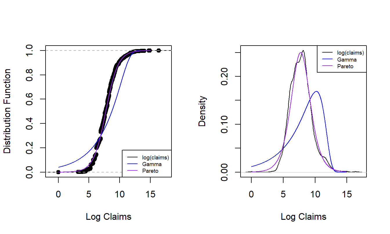
Figure 6.1: Nonparametric Versus Fitted Parametric Distribution and Density Functions. The left-hand panel compares distribution functions, with the dots corresponding to the empiricaldistribution, the thick blue curve corresponding to the fitted gamma and the light purple curve corresponding to the fitted Pareto. The right hand panel compares these three distributions summarized using probability density functions.
For another way to compare the appropriateness of two fitted models, consider the probability-probability (pp) plotA plot that compares two models through their cumulative probabilities.. A \(pp\) plot compares cumulative probabilities under two models. For our purposes, these two models are the nonparametric empirical distribution function and the parametric fitted model. Figure 6.2 shows \(pp\) plots for the Property Fund data introduced in Section 1.3. The fitted gamma is on the left and the fitted Pareto is on the right, compared to the same empirical distribution function of the data. The straight line represents equality between the two distributions being compared, so points close to the line are desirable. As seen in earlier demonstrations, the Pareto is much closer to the empirical distribution than the gamma, providing additional evidence that the Pareto is the better model.
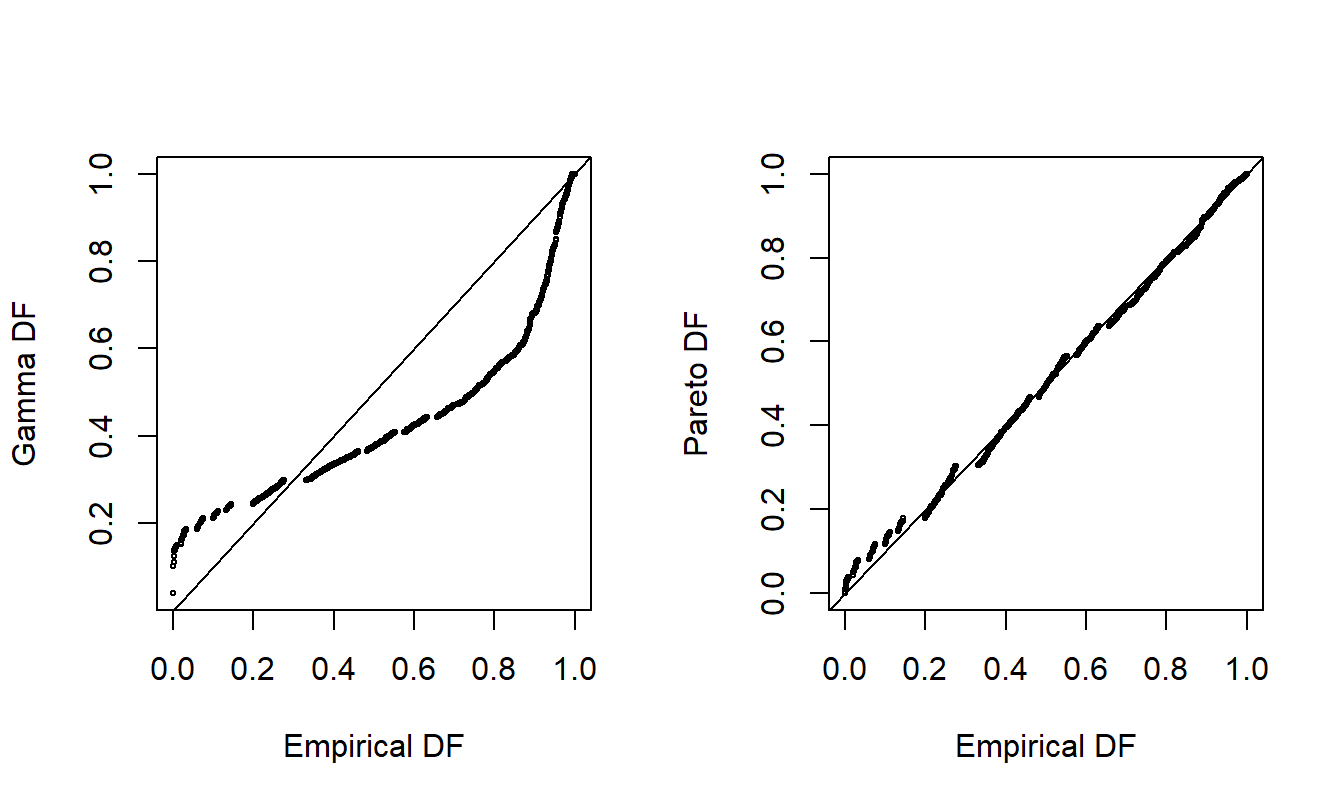
Figure 6.2: Probability-Probability (\(pp\)) Plots. The horizontal axis gives the empirical distribution function at each observation. In the left-hand panel, the corresponding distribution function for the gamma is shown in the vertical axis. The right-hand panel shows the fitted Pareto distribution. Lines of \(y=x\) are superimposed.
A \(pp\) plot is useful in part because no artificial scaling is required, such as with the overlaying of densities in Figure 6.1, in which we switched to the log scale to better visualize the data. The Chapter 6 Technical Supplement A.1 introduces a variation of the \(pp\) plot known as a Lorenz curveA graph of the proportion of a population on the horizontal axis and a distribution function of interest on the vertical axis.; this is an important tool for assessing income inequality. Furthermore, \(pp\) plots are available in multivariate settings where more than one outcome variable is available. However, a limitation of the \(pp\) plot is that, because it plots cumulative distribution functions, it can sometimes be difficult to detect where a fitted parametric distribution is deficient. As an alternative, it is common to use a quantile-quantile (qq) plotA plot that compares two models through their quantiles., as demonstrated in Figure 6.3.
The \(qq\) plot compares two fitted models through their quantiles. As with \(pp\) plots, we compare the nonparametric to a parametric fitted model. Quantiles may be evaluated at each point of the dataset, or on a grid (e.g., at \(0, 0.001, 0.002, \ldots, 0.999, 1.000\)), depending on the application. In Figure 6.3, for each point on the aforementioned grid, the horizontal axis displays the empirical quantile and the vertical axis displays the corresponding fitted parametric quantile (gamma for the upper two panels, Pareto for the lower two). Quantiles are plotted on the original scale in the left panels and on the log scale in the right panels to allow us to see where a fitted distribution is deficient. The straight line represents equality between the empirical distribution and fitted distribution. From these plots, we again see that the Pareto is an overall better fit than the gamma. Furthermore, the lower-right panel suggests that the Pareto distribution does a good job with large claims, but provides a poorer fit for small claims.
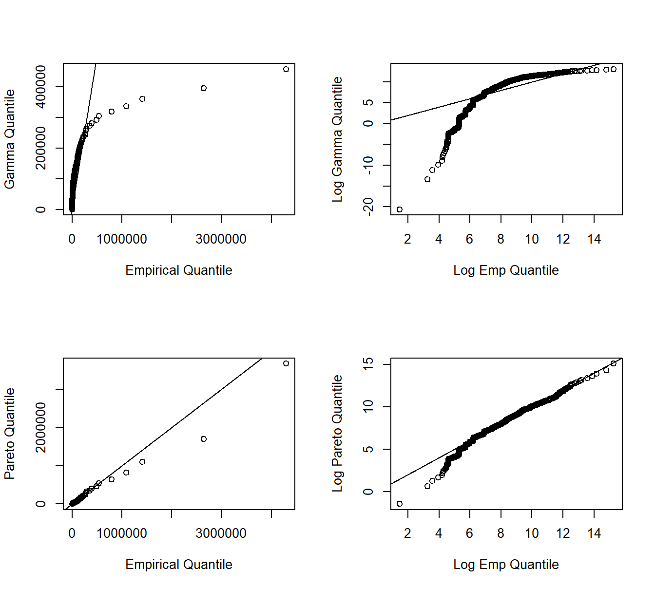
Figure 6.3: Quantile-Quantile (\(qq\)) Plots. The horizontal axis gives the empirical quantiles at each observation. The right-hand panels they are graphed on a logarithmic basis. The vertical axis gives the quantiles from the fitted distributions; gamma quantiles are in the upper panels, Pareto quantiles are in the lower panels.
Example 6.1.1. Actuarial Exam Question. The graph below shows a \(pp\) plot of a fitted distribution compared to a sample.
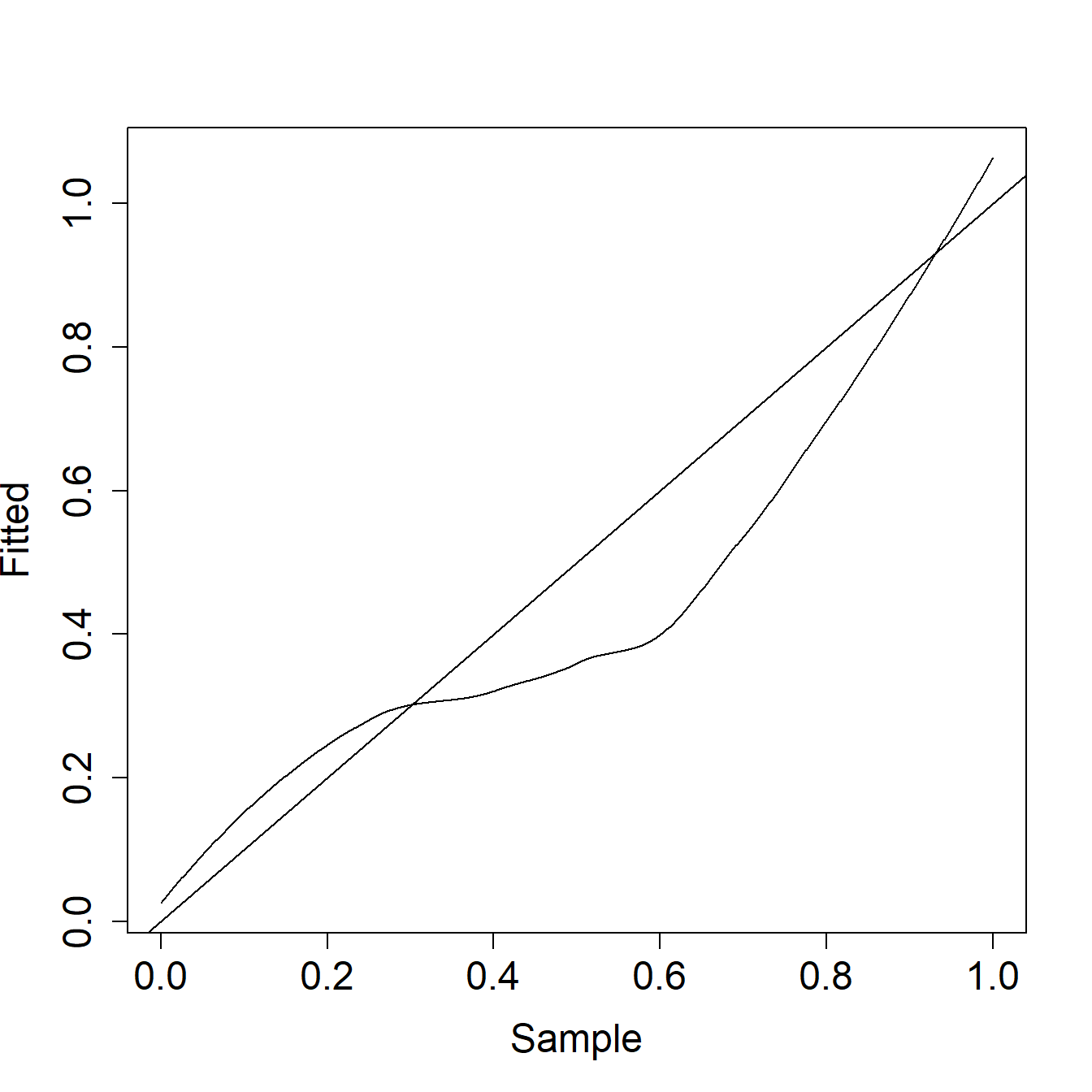
Comment on the two distributions with respect to left tail, right tail, and median probabilities.
Show Example Solution
6.1.2 Statistical Comparison of Distributions
When selecting a model, it is helpful to make the graphical displays presented. However, for reporting results, it can be effective to supplement the graphical displays with selected statistics that summarize model goodness of fit. Table 6.1 provides three commonly used goodness of fit statistics. In this table, \(F_n\) is the empirical distribution, \(F\) is the fitted or hypothesized distribution, and \(F_i^* = F(x_i)\).
Table 6.1. Three Goodness of Fit Statistics
\[ {\small \begin{matrix} \begin{array}{l|cc} \hline \text{Statistic} & \text{Definition} & \text{Computational Expression} \\ \hline \text{Kolmogorov-} & \max_x |F_n(x) - F(x)| & \max(D^+, D^-) \text{ where } \\ ~~~\text{Smirnov} && D^+ = \max_{i=1, \ldots, n} \left|\frac{i}{n} - F_i^*\right| \\ && D^- = \max_{i=1, \ldots, n} \left| F_i^* - \frac{i-1}{n} \right| \\ \text{Cramer-von Mises} & n \int (F_n(x) - F(x))^2 f(x) dx & \frac{1}{12n} + \sum_{i=1}^n \left(F_i^* - (2i-1)/n\right)^2 \\ \text{Anderson-Darling} & n \int \frac{(F_n(x) - F(x))^2}{F(x)(1-F(x))} f(x) dx & -n-\frac{1}{n} \sum_{i=1}^n (2i-1) \log\left(F_i^*(1-F_{n+1-i})\right)^2 \\ \hline \end{array} \\ \end{matrix} } \]
The Kolmogorov-Smirnov statistic is the maximum absolute difference between the fitted distribution function and the empirical distribution function. Instead of comparing differences between single points, the Cramer-von Mises statistic integrates the difference between the empirical and fitted distribution functions over the entire range of values. The Anderson-Darling statistic also integrates this difference over the range of values, although weighted by the inverse of the variance. It therefore places greater emphasis on the tails of the distribution (i.e when \(F(x)\) or \(1-F(x)=S(x)\) is small).
Example 6.1.2. Actuarial Exam Question (modified). A sample of claim payments is:
\[ \begin{array}{ccccc} 29 & 64 & 90 & 135 & 182 \\ \end{array} \]
Compare the empirical claims distribution to an exponential distribution with mean \(100\) by calculating the value of the Kolmogorov-Smirnov test statistic.
Show Example Solution
Show Quiz Solution
6.2 Iterative Model Selection
In our model development, we examine the data graphically, hypothesize a model structure, and compare the data to a candidate model in order to formulate an improved model. Box (1980) describes this as an iterative process which is shown in Figure 6.4.
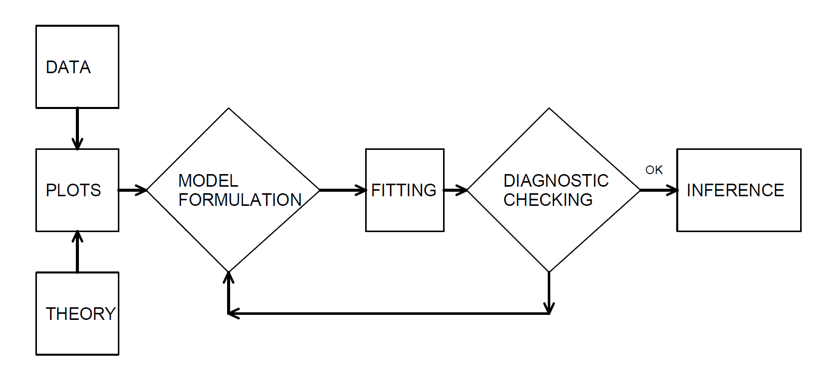
Figure 6.4: Iterative Model Specification Process
This iterative process provides a useful recipe for structuring the task of specifying a model to represent a set of data.
- The first step, the model formulation stage, is accomplished by examining the data graphically and using prior knowledge of relationships, such as from economic theory or industry practice.
- The second step in the iteration is fitting based on the assumptions of the specified model. These assumptions must be consistent with the data to make valid use of the model.
- The third step is diagnostic checking; the data and model must be consistent with one another before additional inferences can be made. Diagnostic checking is an important part of the model formulation; it can reveal mistakes made in previous steps and provide ways to correct these mistakes.
The iterative process also emphasizes the skills you need to make data analytics work. First, you need a willingness to summarize information numerically and portray this information graphically. Second, it is important to develop an understanding of model properties. You should understand how a probabilistic model behaves in order to match a set of data to it. Third, theoretical properties of the model are also important for inferring general relationships based on the behavior of the data.
6.3 Model Selection Based on a Training Dataset
As introduced in Section 2.2, it is common to refer to a dataset used for fitting the model as a training or an in-sample dataset. Techniques available for selecting a model depend upon whether the outcomes \(X\) are discrete, continuous, or a hybrid of the two, although the principles are the same.
Graphical and other Basic Summary Measures. Begin by summarizing the data graphically and with statistics that do not rely on a specific parametric form, as summarized in Section 4.4.1. Specifically, you will want to graph both the empirical distribution and density functions. Particularly for loss data that contain many zeros and that can be skewed, deciding on the appropriate scale (e.g., logarithmic) may present some difficulties. For discrete data, tables are often preferred. Determine sample moments, such as the mean and variance, as well as selected quantiles, including the minimum, maximum, and the median. For discrete data, the mode (or most frequently occurring value) is usually helpful.
These summaries, as well as your familiarity of industry practice, will suggest one or more candidate parametric models. Generally, start with the simpler parametric models (for example, one parameter exponential before a two parameter gamma), gradually introducing more complexity into the modeling process.
Critique the candidate parametric model numerically and graphically. For the graphs, utilize the tools introduced in Section 6.1 such as \(pp\) and \(qq\) plots. For the numerical assessments, examine the statistical significance of parameters and try to eliminate parameters that do not provide additional information. In addition to statistical significance of parameters, you may use the following model comparison tools.
Likelihood Ratio Tests. For comparing model fits, if one model is a subset of another, then a likelihood ratio test may be employed; the general approach to likelihood ratio testing is described in Appendix Sections 17.4.3 and 19.3.2.
Goodness of Fit Statistics. Generally, models are not proper subsets of one another in which case overall goodness of fit statistics are helpful for comparing models. Information criteria are one type of goodness of statistic. The most widely used examples are Akaike’s Information Criterion (AIC) and the (Schwarz) Bayesian Information Criterion (BIC); they are widely cited because they can be readily generalized to multivariate settings. Appendix Section 17.4.4 provides a summary of these statistics.
For selecting the appropriate distribution, statistics that compare a parametric fit to a nonparametric alternative, summarized in Section 6.1.2, are useful for model comparison. For discrete data, a goodness of fit statistic is generally preferred as it is more intuitive and simpler to explain.
6.4 Model Selection Based on a Test Dataset
Model validationThe process of confirming that the proposed model is appropriate. introduced in Section 2.2 is the process of confirming that the proposed model is appropriate based on a test or an out-of-sample dataset, especially in light of the purposes of the investigation. Model validation is important since the model selection process based only on training or in-sample data can be susceptible to data-snoopingRepeatedly fitting models to a data set without a prior hypothesis of interest., that is, fitting a great number of models to a single set of data. By looking at a large number of models, we may overfit the data and understate the natural variation in our representation.
Selecting a model based only on in-sample data also does not support the goal of predictive inferencePreditive inference is the process of using past data observations to predict future observations.. Particularly in actuarial applications, our goal is to make statements about new experience rather than a dataset at hand. For example, we use claims experience from one year to develop a model that can be used to price insurance contracts for the following year. As an analogy, we can think about the training dataset as experience from one year that is used to predict the behavior of the next year’s test dataset.
We can respond to these criticisms by using a technique known as out-of-sample validation. The ideal situation is to have available two sets of data, one for training, or model development, and the other for testing, or model validation. We initially develop one or several models on the first dataset that we call candidate models. Then, the relative performance of the candidate models can be measured on the second set of data. In this way, the data used to validate the model are unaffected by the procedures used to formulate the model.
Random Split of the Data. Unfortunately, rarely will two sets of data be available to the investigator. As mentioned in Section 2.2, we can implement the validation process by splitting the dataset into training and test subsamples, respectively. Figure 6.5 illustrates this splitting of the data.
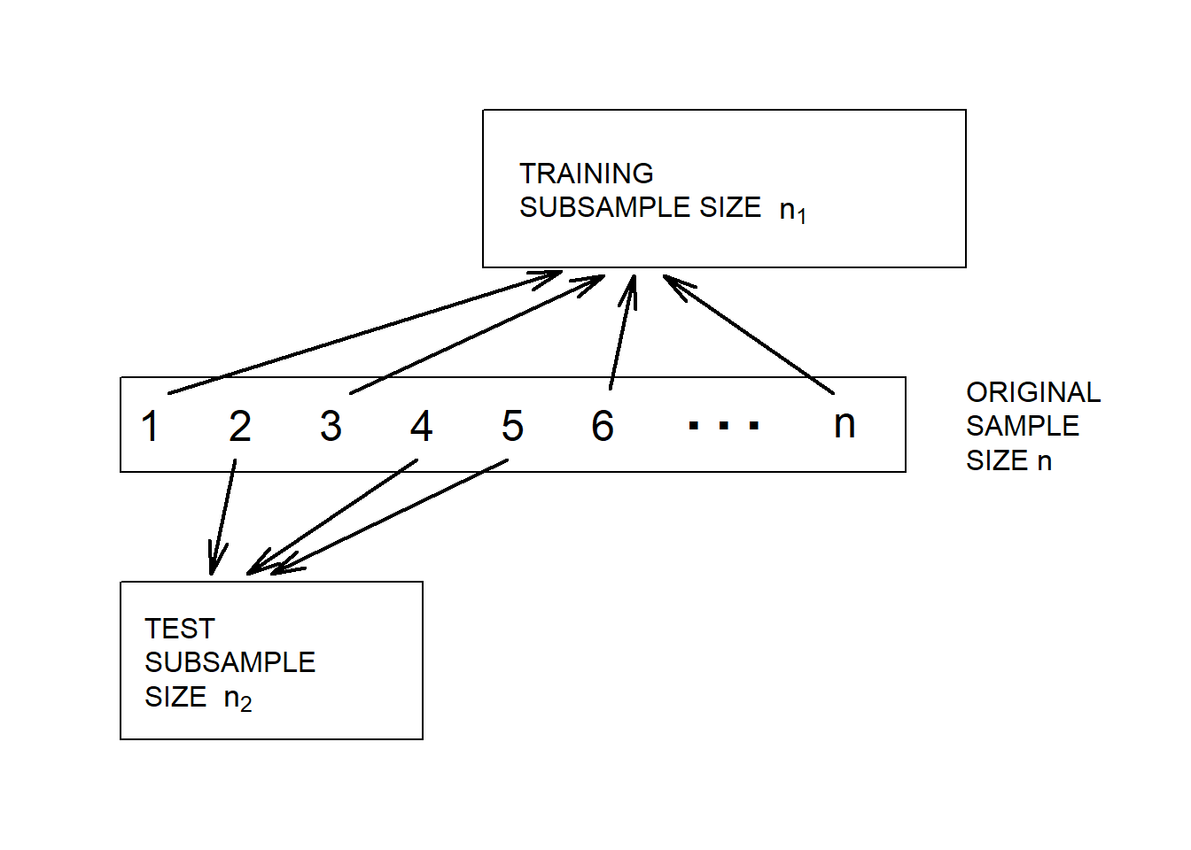
Figure 6.5: Model Validation. A dataset is randomly split into two subsamples.
Various researchers recommend different proportions for the allocation. Snee (1977) suggests that data-splitting not be done unless the sample size is moderately large. The guidelines of Picard and Berk (1990) show that the greater the number of parameters to be estimated, the greater the proportion of observations is needed for the training subsample for model development.
Selecting a Distribution. Still, our focus so far has been to select a distribution for a dataset that can be used for actuarial modeling without additional explanatory or input variables \(x_1, \ldots, x_k\). Even in this more fundamental problem, the model validation approach is valuable. If we base all inference on only in-sample data, then there is a tendency to select more complicated models than needed. For example, we might select a four parameter GB2, generalized beta of the second kind, distribution when only a two parameter Pareto is needed. Information criteria such as AICA goodness of fit measure of a statistical model that describes how well it fits a set of observations. and BICBayesian information criterion introduced in Appendix Section 17.4.4 include penalties for model complexity and thus provide protection against over-fitting, but using a test sample may also help achieve parsimonious models. From a quote often attributed to Albert Einstein, we want to “use the simplest model as possible but no simpler.”
Example 6.4.1. Wisconsin Property Fund. For the 2010 property fund data from Section 1.3, we may try to select a severity distribution based on out-of-sample prediction. In particular, we may randomly select 1,000 observations as our training data, and use the remaining 377 claims to validate the two models based respectively on gamma and Pareto distributions. For illustration purposes, We compare the Kolmogorov-Smirnov statistics respectively for the training and test datasets using the models fitted from training data.
Show R Code for Kolmogorov-Smirnov model validation
Model Validation Statistics. In addition to the nonparametric tools introduced earlier for comparing marginal distributions of the outcome or output variables ignoring potential explanatory or input variables, much of the literature supporting the establishment of a model validation process is based on regression and classification models that you can think of as an input-output problem (James et al. (2013)). That is, we have several inputs or predictor variables \(x_1, \ldots, x_k\) that are related to an output or outcome \(y\) through a function such as \[y = \mathrm{g}\left(x_1, \ldots, x_k\right).\]For model selection, one uses the training sample to develop an estimate of \(\mathrm{g}\), say, \(\hat{\mathrm{g}}\), and then calibrate the average distance from the observed outcomes to the predictions using a criterion of the form
\[\begin{equation} \frac{1}{n}\sum_i \mathrm{d}(y_i,\hat{\mathrm{g}}\left(x_{i1}, \ldots, x_{ik}\right) ) . \tag{6.1} \end{equation}\]Here, “d” is some measure of distance and the sum \(i\) is over the test data. The function \(\mathrm{g}\) may not have an analytical form and can be estimated for each observation using the different different types of algorithms and models introduced earlier in Section 2.4. In many regression applications, it is common to use the squared Euclidean distance of the form \(\mathrm{d}(y_i,\mathrm{g}) = (y_i-\mathrm{g})^2\) under which the criterion in equation (6.1) is called the mean squared error (MSE). Using data simulated from linear models, Example 2.3.1 uses the root mean squared error (Rmse) which is the squared root of the MSE. From equation (6.1), the MSE criteria works the best for linear models under normal distributions with constant variance, as minimizing MSE is equivalent to the maximum likelihood and least squares criterion in training data. In data analytics and linear regression, one may consider transformations of the outcome variable in order for the MSE criteria to work more effectively. In actuarial applications, the mean absolute error (MAE) under the Euclidean distance \(\mathrm{d}(y_i,\mathrm{g}) = |y_i-\mathrm{g}|\) may be preferred because of the skewed nature of loss data. For right-skewed outcomes, it may require a larger sample size for the validation statistics to pickup the correct model when large outlying values of \(y\) can have a large effect on the measures.
Following Example 2.3.1, we use simulated data in Examples 6.4.2 through 6.4.4 to compare the AIC information criteria from Appendix Chapter 17.4.4 with out-of-sample MSE and MAE criterion for selecting the distribution and input variables for outcomes that are respectively from normal and right-skewed distributions including lognormal and gamma distributions. For right skewed distributions, we find that the AIC information criteria seems to work consistently for selecting the correct distributional form and mean structure (input variables), whereas out-of-sample MSE and MAE may not work for right-skewed outcomes like those from gamma distributions, even with relatively large sample sizes. Therefore, model validation statistics commonly used in data analytics may only work for minimizing specific cost functions, such as the MAE that represents the average absolute error for out-of-sample prediction, and do not necessarily guarantee correct selection of the underlying data generating mechanism.
Example 6.4.2. In-sample AIC and out-of-sample MSE for normal outcomes. Example 2.3.1 assumes that there is a set of claims that potentially varies by a single categorical variable with six levels. To illustrating in-sample over-fitting, it also assumes that two of the six levels share a common mean that differs from rest of levels. For Example 2.3.1, the claim amounts were generated from a linear model with constant variance, for which in-sample AIC and out-of-sample Rmse provide consistent results from the cross-validation procedure to be introduced in the next section. Here, we may use the same data generation mechanism to compare the performance of in-sample AIC with the in-sample and out-of-sample Rmse criteria. In particular, we generate a total of 200 samples and split them equally into the training and test datasets. From the output table, we observe the two-level model was correctly selected by both in-sample AIC and out-of-sample MSE criteria, whereas in-sample MSE prefers an over-fitted model with six levels. Thus, due to concerns of model over-fitting, we do not use in-sample distance measures such as the MSE and MAE criterion that favors more complicated models.
Show R Code for model validation statistics
Example 6.4.3. MSE and MAE for right-skewed outcomes - lognormal claims. For claims modeling, one may wonder how the MSE and MAE types of criterion may perform for right-skewed data. Using the same data generating procedure, we may generate lognormal claim amounts by exponentiating the normal outcomes from the previous example. We fit the lognormal claim amounts with gamma and lognormal regression commonly used for ratemaking and claims analytics. For the specific data generating mechanism, we observe that it requires a larger sample size for out-of-sample Rmse and MAE to select the correct distributional form and mean structure, when compared with in-sample AIC criteria. The AIC criteria is able to pick out the correct model with a sample size of 200, while out-of-sample MSE and MAE fail to. Thus, for right skewed output, precautions need to be taken when using model validation statistics that may be sensitive to large claim values, particularly when the sample size is relatively small.
Show R Code for model validation statistics for lognormal outputs
Example 6.4.4. MSE and MAE for right-skewed outcomes - gamma claims. For right-skewed outcomes, we may be interested in studying how the MSE and MAE types of measures work for another loss severity distribution, the gamma distribution, that is widely used in ratemaking and claims analytics. Here, we use a similar mean structure for generating claims amounts based on a gamma regression with the log link function. We fit the data using gamma regression and lognormal regression. For gamma outcomes, the table shows that out-of-sample MSE and MAE criterion fail to select the correct distributional form or the mean structure even with a total of 1000 samples. By changing the gamma shape parameter, you may see that the out-of-sample MSE and MAE criterion work in certain settings for correctly selecting the distributional form or the mean structure, but the performance of such model validation statistics does not seem to be consistent across different parameter values and sample sizes for right-skewed gamma outcomes. Again, the AIC criteria seems to be working consistently in selecting the correct distribution and mean structure for the data generated from gamma distributions, even with a smaller sample size of 200.
Show R Code for model validation statistics for gamma outputs
Chapter 10 describes another measure, the Gini indexA measure for assessing income inequality. it measures the discrepancy between the income and population distributions and is calculated from the lorenz curve., that may be useful in actuarial applications particularly when there is a large proportion of zeros in claims data (corresponding to no claims) that may invalidate the aforementioned model validation statistics.
6.5 Model Selection Based on Cross-Validation
Although out-of-sample validation is the gold standard in predictive modeling, it is not always practical to do so. The main reason is that we have limited sample sizes and the out-of-sample model selection criterion in equation (6.1) depends on a random split of the data. This means that different analysts, even when working the same dataset and same approach to modeling, may select different models. This is likely in actuarial applications because we work with skewed datasets where there is a large chance of getting some very large outcomes and large outcomes may have a great influence on the parameter estimates.
Cross-Validation Procedure. Alternatively, one may use cross-validation, as follows.
- The procedure begins by using a random mechanism to split the data into \(K\) subsets of roughly equal size known as folds, where analysts typically use 5 to 10.
- Next, one uses the first \(K\)-1 subsamples to estimate model parameters. Then, “predict” the outcomes for the \(K\)th subsample and use a measure such as in equation (6.1) to summarize the fit.
- Now, repeat this by holding out each of the \(K\) subsamples, summarizing with an out-of-sample statistic. Thus, summarize these \(K\) statistics, typically by averaging, to give a single overall statistic for comparison purposes.
Repeat these steps for several candidate models and choose the model with the lowest overall cross-validation statistic.
In Example 2.3.1, you have seen that the MSE criteria seems to work with k-fold cross-validation in selecting the correct mean structure for claims outcome data generated from linear models with constant variance. From Examples 6.4.3 and 6.4.4, however, the out-of-sample MSE and MAE criterion does not seem to provide consistent performance for selecting the distributional form and the mean structure under right-skewed claims distributions. Thus, we may use the k-folder cross-validation instead of out-of-sample prediction to see whether the MSE and MAE types of criterion work for right-skewed distributions based on lognormal and gamma regression with a log link function.
Example 6.5.1. Cross-validation in right-skewed outcomes - lognormal claims For lognormal claims, we use the data generating mechanism from Example 6.4.3 to generate a total of 100 samples, and use the k-fold cross validation procedure in Example 2.3.1 to select the distributional form and mean structure. Using cross-validation, we note that both AIC and out-of-sample MSE and MAE seem to be working for selecting the model with the correct distribution and mean structure, even with a total of 100 samples.
Show R Code for cross-validation with lognormal outputs
Example 6.5.2. Cross-validation in right-skewed outcomes - gamma claims For gamma claims, we use the data generating mechanism from Example 6.4.4 to generate a total of 100 samples, and use the k-fold cross validation procedure to select the distributional form and mean structure. Using cross-validation, we note that in-sample AIC seems to be working for selecting the model with the correct distribution and mean structure, while out-of-sample MSE and MAE seem to fail in selecting the distributional form or the mean structure correctly even after we increase the sample size to 1000.
Show R Code for cross-validation with gamma outputs
Cross-validation is widely used because it retains the predictive flavor of the out-of-sample model validation process but, due to the re-use of the data, is more stable over random samples. In addition, Example 8.3.1 in Chapter 8 uses the Wisconsin Property Fund to perform k-fold cross-validation of the gamma and Pareto models based on the Kolmogorov-Smirnov goodness of fit statistic. Additional information and examples regarding re-sampling procedures including leave-one-out cross-validation and bootstrap can also be found in Chapter 8.
6.6 Model Selection for Modified Data
So far, you have learned covered model selection using unmodified data. For modified data including grouped, censored and truncated data, you have learned parametric and nonparametric estimation of distribution functions in Section 5.2. For model selection, the tools from Section 6.1 can be extended to cases of modified data.
For selection of distributions, the nonparametric tools introduced in Section 6.1 are based on estimated parametric and nonparametric distribution functions, and thus can be extended to modified data for which both types of estimators exist.
For graphical comparisons, the \(pp\) and \(qq\) plots introduced earlier
can be created for modified data by plotting the parametric estimates
from Section 5.2 against nonparametric estimates
of the probability or distribution functions from Section
5.3. For example, the qqPlotCensored and
qqtrunc functions in R generate \(qq\) plots respectively for censored
(left or right) and truncated data, whereas the probPlot function
creates both \(pp\) and \(qq\) plots with a larger selection of
distributions for right-censored and unmodified data. Additional
graphical tools such as cumulative hazard plots are available in the R
package GofCens.
Example 6.6.1. Bodily Injury Claims. For the Boston auto bodily injury claims data from Example 5.3.2, we include the full dataset with right-censoring, and use the \(qq\)-plot to compare the estimated quantiles from lognormal, normal and exponential distributions with those from the nonparametric Kaplan-Meier method. From the \(qq\)-plots in Figure ??, the lognormal distribution functions seems to fit the censored data much better those based on the normal and exponential distributions.
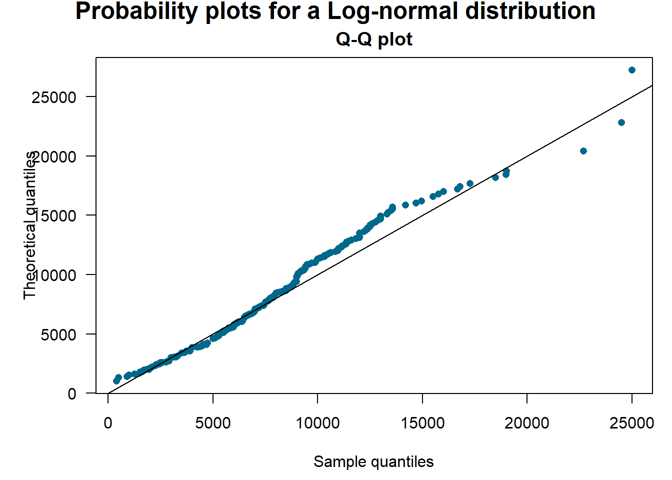
Figure 6.6: Quantile-Quantile (\(qq\)) Plots for Bodily Injury Claims. The horizontal axis gives the empirical quantiles at each observation. The vertical axis gives the quantiles from the fitted distributions; lognormal quantiles are in the left panels, normal quantiles are in the right panels.
$Distribution
[1] "Log-normal"

$Parameters
 location     scale
8.7479091 0.6406153 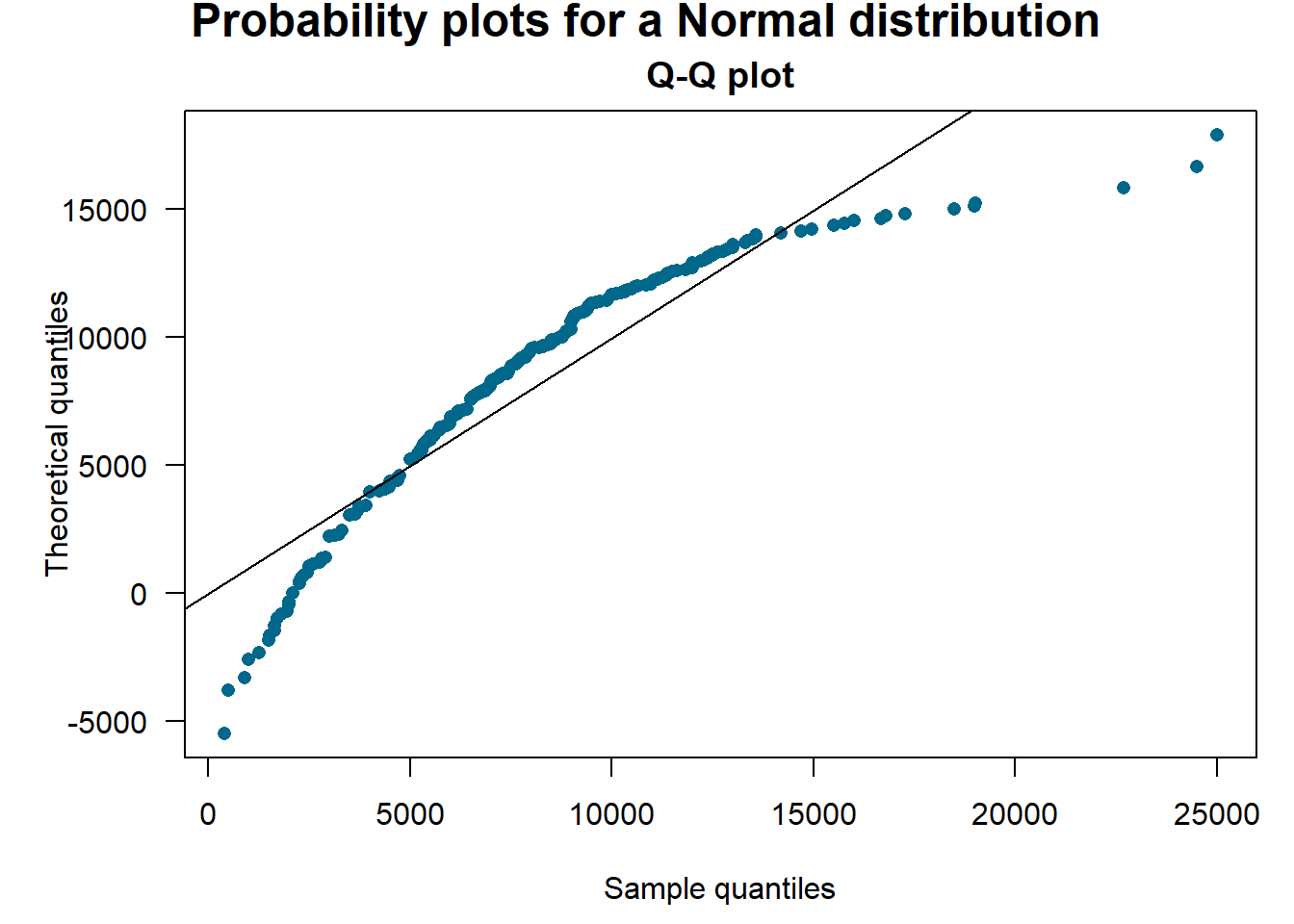
Figure 6.7: Quantile-Quantile (\(qq\)) Plots for Bodily Injury Claims. The horizontal axis gives the empirical quantiles at each observation. The vertical axis gives the quantiles from the fitted distributions; lognormal quantiles are in the left panels, normal quantiles are in the right panels.
$Distribution
[1] "Normal"

$Parameters
location    scale
7463.069 4575.343 
Figure 6.8: Quantile-Quantile (\(qq\)) Plots for Bodily Injury Claims. The horizontal axis gives the empirical quantiles at each observation. The vertical axis gives the quantiles from the fitted distributions; lognormal quantiles are in the left panels, normal quantiles are in the right panels.
$Distribution
[1] "Exponential"

$scale
[1] 7710.53
Show R Code
In addition to graphical tools, you may use tools from Section
6.1.2 for statistical comparisons of models fitted
from modified data based on parametric and nonparametric estimates of
distribution functions. For example, the R package GofCens provides
functions calculating the three goodness of fit statistics from Section
6.1.2 for both right-censored and unmodified data. The
R package truncgof, on the other hand, provides functions for
calculating the three goodness of fit statistics for left-truncated
data.
Example 6.6.2. Bodily Injury Claims. For the Boston auto bodily injury claims with right-censoring, we may use the goodness of fit statistics to evaluate the fitted lognormal, normal and exponential distributions. For the Kolmogorov-Smirnov, Cramer-von Mises and Anderson-Darling statistics, the lognormal distribution gives values that are much lower than those from normal and exponential distributions. The conclusion from the goodness of fit statistics is consistent to that revealed by the \(qq\) plots.
| Kolmogorov-Smirnov | Cramer-von Mises | Anderson-Darling | |
|---|---|---|---|
| Lognormal | 1.994 | 0.304 | 1.770 |
| Normal | 3.096 | 1.335 | 9.437 |
| Exponential | 4.811 | 4.065 | 21.659 |
Show R Code
Other than selecting the distributional form, model comparison measures
such as the likelihood ratio test and information criterion including
the AIC from Section 6.3 can be obtained
for models fitted based on likelihood criteria based on the likelihood
functions introduced earlier for modified data. For modified data, the
survreg and flexsurvreg functions in R fit parametric regression
models on censored and/or truncated outcomes based on maximum likelihood
estimation which allows use of likelihood ratio tests and information
criterion such as AIC for in-sample model comparisons. For censored and
truncated data, the functions also provide output of residuals that
allow calculation of model validation statistics such as the MSE and MAE
for the iterative model selection procedure introduced in Section
6.2.
Show Quiz Solution
6.7 Further Resources and Contributors
Exercises
Here are a set of exercises that guide the viewer through some of the theoretical foundations of Loss Data Analytics. Each tutorial is based on one or more questions from the professional actuarial examinations, typically the Society of Actuaries Exam C/STAM.
Contributors
- Lei (Larry) Hua and **Michelle Xia*, Northern Illinois University, are the principal authors of the second edition of this chapter.
- Edward W. (Jed) Frees and Lisa Gao, University of Wisconsin-Madison, are the principal authors of the initial version of this chapter. Email:jfrees@bus.wisc.edu for chapter comments and suggested improvements.
- Chapter reviewers include: Vytaras Brazauskas, Yvonne Chueh, Eren Dodd, Hirokazu (Iwahiro) Iwasawa, Joseph Kim, Andrew Kwon-Nakamura, Jiandong Ren, and Di (Cindy) Xu.