Chapter 5 Modeling Claim Severity

Chapter Preview. In Chapter 4 we explored the use of continuous as well as mixture distributions to model the random size of loss. Often the risk of loss is shared between the policyholder (the insured) and the insurer. Sharing risk can take the form of a deductible that is paid out-of-pocket of the insured before the insurer contributes to the loss, the form of a limit that caps the insured’s liability for loss to a certain amount, or the form of a portion of the loss the insurer is responsible for covering after the insured covers his/her share of the cost, among other forms of cost-sharing. In Sections 5.1.1 to 5.1.3 we introduce the policy deductible feature of the insurance contract, the limited policy, and the co-insurance cost-sharing arrangement. In Section 5.1.4 we explore how insurance companies transfer part of the underlying insured risk by securing coverage from a reinsurer. Section 5.2 covers parametric estimation methods for modified data including grouped, censored and truncated data. In Section 5.3 we apply some non-parametric estimation tools like the ogive estimator, the plug-in principle, the Kaplan-Meier product-limit estimator, and the Nelson Aalon estimator on the modified data.

5.1 Coverage Modifications

---

In this section, you learn how to:

• Describe the policy deductible feature of the insurance contract, the limited policy, and the coinsurance factor.
• Describe the distinction between the loss incurred to the insured and the amount of paid claim by the insurer under different policy modifications.
• Derive the distribution functions and raw moments for the amount of paid claim by the insurer for the different insurance contracts.
• Calculate the percentage decrease in the expected payment of the insurer as a result of imposing the deductible.
• Describe the insurance mechanism for insurance companies (reinsurance).
• Calculate the raw moments of the amount retained by the primary insurer in the reinsurance agreement.

---

In this section we evaluate the impacts of coverage modifications: a) deductibles, b) policy limit, c) coinsurance and d) inflation on insurer’s costs.

5.1.1 Policy Deductibles

Under an ordinary deductible policy, the insured (policyholder) agrees to cover a fixed amount of an insurance claim before the insurer starts to pay. This fixed expense paid out of pocket is called the deductible and often denoted by \(d\). If the loss exceeds \(d\) then the insurer is responsible for covering the loss X less the deductible \(d\). Depending on the agreement, the deductible may apply to each covered loss or to the total losses during a defined benefit period (such as a month, year, etc.)

Deductibles reduce premiums for the policyholders by eliminating a large number of small claims, the costs associated with handling these claims, and the potential moral hazardSituation where an insured is more likely to be risk seeking if they do not bear sufficient consequences for a loss arising from having insurance. Moral hazard occurs when the insured takes more risks, increasing the chances of loss due to perils insured against, knowing that the insurer will incur the cost (e.g. a policyholder with collision insurance may be encouraged to drive recklessly). The larger the deductible, the less the insured pays in premiums for an insurance policy.

Let \(X\) denote the loss incurred to the insured and \(Y\) denote the amount of paid claim by the insurer. Speaking of the benefit paid to the policyholder, we differentiate between two variables: The payment per loss and the payment per payment. The payment per lossAmount insurer pays when a loss occurs and can be 0 variable, denoted by \(Y^{L}\) or \((X-d)_+\) is left censoredValues below a threshold d are not ignored but converted to 0 because values of \(X\) that are less than \(d\) are set equal to zero. This variable is defined as

\[ Y^{L} = \left( X - d \right)_{+} = \left\{ \begin{array}{cc} 0 & X \le d, \\ X - d & X > d \end{array} \right. . \] \(Y^{L}\) is often referred to as left censored and shifted variable because the values below \(d\) are not ignored and all losses are shifted by a value \(d\).

On the other hand, the payment per paymentAmount insurer pays given a payment is needed and is greater than 0 variable, denoted by \(Y^{P}\), is defined only when there is a payment. Specifically, \(Y^P\) equals \(X-d\) on the event \(\{X >d\}\), denoted as \(Y^P = X-d ||X>d\). Another way of expressing this that is commonly used is

\[ Y^{P} = \left\{ \begin{matrix} \text{Undefined} & X \le d \\ X - d & X > d . \end{matrix} \right. \]

Here, \(Y^{P}\) is often referred to as left truncatedValues below a threshold d are not reported and unknown and shifted variable or excess loss variable because the claims smaller than \(d\) are not reported and values above \(d\) are shifted by \(d\).

Even when the distribution of \(X\) is continuous, the distribution of \(Y^{L}\) is a hybrid combination of discrete and continuous components. The discrete part of the distribution is concentrated at \(Y = 0\) (when \(X \leq d\)) and the continuous part is spread over the interval \(Y > 0\) (when \(X > d\)). For the discrete part, the probability that no payment is made is the probability that losses fall below the deductible; that is, \[\Pr\left( Y^{L} = 0 \right) = \Pr\left( X \leq d \right) = F_{X}\left( d \right).\] Using the transformation \(Y^{L} = X - d\) for the continuous part of the distribution, we can find the pdf of \(Y^{L}\) given by

\[ f_{Y^{L}}\left( y \right) = \left\{ \begin{matrix} F_{X}\left( d \right) & y = 0 \\ f_{X}\left( y + d \right) & y > 0 . \end{matrix} \right. \]

We can see that the payment per payment variable is the payment per loss variable (\(Y^P= Y^L\)) conditional on the loss exceeding the deductible (\(X > d\)); that is, \(Y^{P} = \left. \ Y^{L} \right|X > d\).. Alternatively, it can be expressed as \(Y^P = (X - d)|X > d\), that is, \(Y^P\) is the loss in excess of the deductible given that the loss exceeds the deductible. Hence, the pdf of \(Y^{P}\) is given by

\[ f_{Y^{P}}\left( y \right) = \frac{f_{X}\left( y + d \right)}{1 - F_{X}\left( d \right)}, \]

for \(y > 0\). Accordingly, the distribution functions of \(Y^{L}\)and \(Y^{P}\) are given by

\[ F_{Y^{L}}\left( y \right) = \left\{ \begin{matrix} F_{X}\left( d \right) & y = 0 \\ F_{X}\left( y + d \right) & y > 0, \\ \end{matrix} \right.\ \]

and

\[ F_{Y^{P}}\left( y \right) = \frac{F_{X}\left( y + d \right) - F_{X}\left( d \right)}{1 - F_{X}\left( d \right)}, \]

for \(y > 0\), respectively.

The raw moments of \(Y^{L}\) and \(Y^{P}\) can be found directly using the pdf of \(X\) as follows \[\mathrm{E}\left\lbrack \left( Y^{L} \right)^{k} \right\rbrack = \int_{d}^{\infty}\left( x - d \right)^{k}f_{X}\left( x \right)dx ,\] and \[ \mathrm{E}\left\lbrack \left( Y^{P} \right)^{k} \right\rbrack = \frac{\int_{d}^{\infty}\left( x - d \right)^{k}f_{X}\left( x \right) dx }{{1 - F}_{X}\left( d \right)} = \frac{\mathrm{E}\left\lbrack \left( Y^{L} \right)^{k} \right\rbrack}{{1 - F}_{X}\left( d \right)}, \] respectively. For \(k=1\), we can use the survival function to calculate \(\mathrm{E}(Y^L)\) as \[ \mathrm{E}(Y^L) = \int_d^{\infty} [1-F_X(x)] ~dx . \] This could be easily proved if we start with the initial definition of \(\mathrm{E}(Y^L)\) and use integration by parts.

We have seen that the deductible \(d\) imposed on an insurance policy is the amount of loss that has to be paid out of pocket before the insurer makes any payment. The deductible \(d\) imposed on an insurance policy reduces the insurer’s payment. The loss elimination ratio (LER)% decrease of the expected payment by the insurer as a result of the deductible is the percentage decrease in the expected payment of the insurer as a result of imposing the deductible. It is defined as \[LER = \frac{\mathrm{E}\left( X \right) - \mathrm{E}\left( Y^{L} \right)}{\mathrm{E}\left( X \right)}.\]

A little less common type of policy deductible is the franchise deductible. The franchise deductibleInsurer pays nothing for losses below the deductible, but pays the full amount for any loss above the deductible will apply to the policy in the same way as ordinary deductible except that when the loss exceeds the deductible \(d\), the full loss is covered by the insurer. The payment per loss and payment per payment variables are defined as \[Y^{L} = \left\{ \begin{matrix} 0 & X \leq d, \\ X & X > d, \\ \end{matrix} \right.\ \] and \[Y^{P} = \left\{ \begin{matrix} \text{Undefined} & X \leq d, \\ X & X > d, \\ \end{matrix} \right.\ \] respectively.

Example 5.1.1. Actuarial Exam Question. A claim severity distribution is exponential with mean 1000. An insurance company will pay the amount of each claim in excess of a deductible of 100. Calculate the variance of the amount paid by the insurance company for one claim, including the possibility that the amount paid is 0.

Show Example Solution

Solution.

Let \(Y^{L}\) denote the amount paid by the insurance company for one claim. \[Y^{L} = \left( X - 100 \right)_{+} = \left\{ \begin{matrix} 0 & X \leq 100, \\ X - 100 & X > 100. \\ \end{matrix} \right.\ \] The first and second moments of \(Y^{L}\) are \[E\left( Y^{L} \right) = \int_{100}^{\infty}\left( x - 100 \right)f_{X}\left( x \right)dx \\ = {\int_{100}^{\infty}{S_{X}\left( x \right)}dx = 1000e}^{- \frac{100}{1000}},\] and \[E\left\lbrack \left( Y^{L} \right)^{2} \right\rbrack = \int_{100}^{\infty}\left( x - 100 \right)^{2}f_{X}\left( x \right)dx \\\\ = 2 \times 1000^{2}e^{- \frac{100}{1000}}.\] So, \[\mathrm{Var}\left( Y^{L} \right) = \left( 2 \times 1000^{2}e^{- \frac{100}{1000}} \right) - \left( {1000e}^{- \frac{100}{1000}} \right)^{2} = 990,944.\]

An arguably simpler path to the solution is to make use of the relationship between \(X\) and \(Y^{P}\). If \(X\) is exponentially distributed with mean 1000, then \(Y^{P}\) is also exponentially distributed with the same mean, because of the memoryless property of the exponential distribution. Hence, \(E\left( Y^{P} \right)\)=1000 and \[E\left\lbrack \left( Y^{P} \right)^{2} \right\rbrack = 2 \times 1000^{2}.\] Using the relationship between \(Y^{L}\) and \(Y^{P}\) we find \[E\left( Y^{L} \right) = \ E\left( Y^{P} \right)S_{X}\left( 100 \right){= 1000e}^{- \frac{100}{1000}}\]

\[E\left\lbrack \left( Y^{L} \right)^{2} \right\rbrack = E\left\lbrack \left( Y^{P} \right)^{2} \right\rbrack S_{X}\left( 100 \right) = 2 \times 1000^{2}e^{- \frac{100}{1000}}.\]

The relationship between \(X\) and \(Y^P\) can also be used when dealing with the uniform or the Pareto distributions. You can easily show that if \(X\) is uniform over the interval \(\left(0,\theta\right)\) then \(Y^P\) is uniform over the interval \(\left(0,\theta-d\right)\) and if \(X\) is Pareto with parameters \(\alpha\) and \(\theta\) then \(Y^P\) is Pareto with parameters \(\alpha\) and \(\theta+d\).

---

Example 5.1.2. Actuarial Exam Question. For an insurance:

• Losses have a density function \[f_{X}\left( x \right) = \left\{ \begin{matrix} 0.02x & 0 < x < 10, \\ 0 & \text{elsewhere.} \\ \end{matrix} \right. \]
• The insurance has an ordinary deductible of 4 per loss.
• \(Y^{P}\) is the claim payment per payment random variable.

Calculate \(\mathrm{E}\left( Y^{P} \right)\).

Show Example Solution

Solution.

We define \(Y^P\) as follows \[ Y^{P} = \left\{ \begin{matrix} \text{Undefined} & X \leq 4, \\ X - 4 & X > 4. \\ \end{matrix} \right.\ \]

So, \(E\left( Y^{P} \right) = \frac{\int_{4}^{10}\left( x - 4 \right)0.02xdx}{{1 - F}_{X}\left( 4 \right)} = \frac{2.88}{0.84} = 3.43\).

Note that we divide by \(S_X(4)=1-F_X(4)\), as this is the probability where the variable \(Y^P\) is defined.

---

Example 5.1.3. Actuarial Exam Question. You are given:

• Losses follow an exponential distribution with the same mean in all years.
• The loss elimination ratio this year is 70%.
• The ordinary deductible for the coming year is 4/3 of the current deductible.

Compute the loss elimination ratio for the coming year.

Show Example Solution

Solution.

Let the losses \(X\sim Exp(\theta)\) and the deductible for the coming year \(d' = \frac{4}{3}d\), the deductible of the current year. The LER for the current year is \[\frac{E\left( X \right) - E\left( Y^{L} \right)}{E\left( X \right)} = \frac{\theta - \theta e^{- d / \theta}}{\theta} = 1 - e^{- d / \theta} = 0.7.\] Then, \(e^{- d / \theta} = 0.3\).

The LER for the coming year is

\[ \begin{array}{ll} &\frac{\theta - \theta \exp(- \frac{d'}{\theta})}{\theta}=\frac{\theta - \theta \exp\left(- \frac{ \frac{4}{3}d }{\theta}\right)}{\theta} \\ &= 1 - \exp\left(- \frac{ \frac{4}{3} d }{\theta}\right) = 1 - \left( e^{-d /\theta} \right)^{4/3} = 1 - {0.3}^{4/3} = 0.8 . \end{array} \]

---

5.1.2 Policy Limits

Under a limited policy, the insurer is responsible for covering the actual loss \(X\) up to the limit of its coverage. This fixed limit of coveragePolicy limit, or maximum contractual financial obligation of the insurer for a loss is called the policy limit and often denoted by \(u\). If the loss exceeds the policy limit, the difference \(X - u\) has to be paid by the policyholder. While a higher policy limit means a higher payout to the insured, it is associated with a higher premium.

Let \(X\) denote the loss incurred to the insured and \(Y\) denote the amount of paid claim by the insurer. The variable \(Y\) is known as the limited loss variable and is denoted by \(X \land u\). It is a right censored variableValues above a threshold u are not ignored but converted to u because values above \(u\) are set equal to \(u\). The limited loss random variable \(Y\) is defined as

\[ Y = X \land u = \left\{ \begin{matrix} X & X \leq u \\ u & X > u. \\ \end{matrix} \right.\ \]

It can be seen that the distinction between \(Y^{L}\) and \(Y^{P}\) is not needed under limited policy as the insurer will always make a payment.

Using the definitions of \(\left(X-u\right)_+ \text{ and } \left(X\land u\right)\), it can be easily seen that the expected payment without any coverage modification, \(X\), is equal to the sum of the expected payments with deductible \(u\) and limit \(u\). That is, \({X=\left(X-u\right)}_++ \left(X\land u\right)\).

When a loss is subject to a deductible \(d\) and a limit \(u\), the per-loss variable \(Y^L\) is defined as \[ Y^{L} = \left\{ \begin{matrix} 0 & X \leq d \\ X - d & d < X \leq u \\ u - d & X > u. \\ \end{matrix} \right.\ \] Hence, \(Y^L\) can be expressed as \(Y^L=\left(X\land u\right)-\left(X\land d\right)\).

Even when the distribution of \(X\) is continuous, the distribution of \(Y\) is a hybrid combination of discrete and continuous components. The discrete part of the distribution is concentrated at \(Y = u\) (when \(X > u\)), while the continuous part is spread over the interval \(Y < u\) (when \(X \leq u\)). For the discrete part, the probability that the benefit paid is \(u\), is the probability that the loss exceeds the policy limit \(u\); that is, \[\Pr \left( Y = u \right) = \Pr \left( X > u \right) = {1 - F}_{X}\left( u \right).\] For the continuous part of the distribution \(Y = X\), hence the pdf of \(Y\) is given by

\[ f_{Y}\left( y \right) = \left\{ \begin{matrix} f_{X}\left( y \right) & 0 < y < u \\ 1 - F_{X}\left( u \right) & y = u. \\ \end{matrix} \right.\ \]

Accordingly, the distribution function of \(Y\) is given by

\[ F_{Y}\left( y \right) = \left\{ \begin{matrix} F_{X}\left( x \right) & 0 < y < u \\ 1 & y \geq u. \\ \end{matrix} \right.\ \]

The raw moments of \(Y\) can be found directly using the pdf of \(X\) as follows \[ \mathrm{E}\left( Y^{k} \right) = \mathrm{E}\left\lbrack \left( X \land u \right)^{k} \right\rbrack = \int_{0}^{u}x^{k}f_{X}\left( x \right)dx + \int_{u}^{\infty}{u^{k}f_{X}\left( x \right)} dx \\ = \int_{0}^{u}x^{k}f_{X}\left( x \right)dx + u^{k}\left\lbrack {1 - F}_{X}\left( u \right) \right\rbrack . \]

An alternative expression using the survival function is

\[ \mathrm{E}\left[ \left( X \land u \right)^{k} \right] = \int_{0}^{u} k x^{k-1} \left[1 - F_{X}(x) \right] dx . \]

In particular, for \(k=1\), this is

\[ \mathrm{E}\left( Y \right) = \mathrm{E}\left( X \land u \right) = \int_{0}^{u} [1-F_{X}(x) ]dx . \] This could be easily proved if we start with the initial definition of \(\mathrm{E}\left( Y \right)\) and use integration by parts. Alternatively, see the following justification of this limited expectation result.

Show the Justification of Limited Expectation Result

\[ \begin{array}{ll} \mathrm{E}\left[ \left( X \wedge u \right)^{k} \right] & = \mathrm{E}\left[ \int_{0}^{X \wedge u} k x^{k-1} dx \right] \\ & = \mathrm{E}\left[ \int_{0}^{u} k x^{k-1} I(X > x) dx \right] \\ & = \int_{0}^{u} k x^{k-1} \mathrm{E} I(X > x) dx \\ &= \int_{0}^{u} k x^{k-1} \left[1 - F_{X}(x) \right] dx . \end{array} \]

This approach uses the Fubini-Tonelli theorem to exchange the expectation and integration. Note that it does not make any continuity assumptions about the distribution of \(X\).

---

Example 5.1.4. Actuarial Exam Question. Under a group insuranceInsurance provided to groups of people to take advantage of lower administrative costs vs. individual policies policy, an insurer agrees to pay 100% of the medical bills incurred during the year by employees of a small company, up to a maximum total of one million dollars. The total amount of bills incurred, \(X\), has pdf

\[ f_{X}\left( x \right) = \left\{ \begin{matrix} \frac{x\left( 4 - x \right)}{9} & 0 < x < 3 \\ 0 & \text{elsewhere.} \\ \end{matrix} \right.\ \]

where \(x\) is measured in millions. Calculate the total amount, in millions of dollars, the insurer would expect to pay under this policy.

Show Example Solution

Solution.

Define the total amount of bills paid by the insurer as \[ Y = X \land 1 = \left\{ \begin{matrix} X & X \leq 1 \\ 1 & X > 1. \\ \end{matrix} \right.\ \]

So \(\mathrm{E}\left( Y \right) = \mathrm{E}\left( X \land 1 \right) = \int_{0}^{1}\frac{x^{2}(4 - x)}{9}dx + 1 \cdot \int_{1}^{3}\frac{x\left( 4 - x \right)}{9}dx = 0.935\).

---

5.1.3 Coinsurance and Inflation

As we have seen in Section 5.1.1, the amount of loss retained by the policyholder can be losses up to the deductible \(d\). The retained loss can also be a percentage of the claim. The percentage \(\alpha\), often referred to as the coinsurance factor, is the percentage of claim the insurance company is required to cover. If the policy is subject to an ordinary deductible and policy limit, coinsurance refers to the percentage of claim the insurer is required to cover, after imposing the ordinary deductible and policy limit. The payment per loss variable, \(Y^{L}\), is defined as \[ Y^{L} = \left\{ \begin{matrix} 0 & X \leq d, \\ \alpha\left( X - d \right) & d < X \leq u, \\ \alpha\left( u - d \right) & X > u. \\ \end{matrix} \right.\ \] The maximum amount paid by the insurer in this case is \(\alpha\left( u - d \right)\), while \(u\) is the maximum covered loss.

We have seen in Section 5.1.2 that when a loss is subject to both a deductible \(d\) and a limit \(u\) the per-loss variable \(Y^L\) can be expressed as \(Y^L=\left(X\land u\right)-\left(X\land d\right)\). With coinsurance, this becomes \(Y^L\) can be expressed as \(Y^L=\alpha\left[(X\land u)-(X\land d)\right]\).

The \(k\)-th raw moment of \(Y^{L}\) is given by \[ \mathrm{E}\left\lbrack \left( Y^{L} \right)^{k} \right\rbrack = \int_{d}^{u}\left\lbrack \alpha\left( x - d \right) \right\rbrack^{k}f_{X}\left( x \right)dx + \left\lbrack \alpha\left( u - d \right) \right\rbrack^{k} [1-F_{X}\left( u \right)] . \]

A growth factorMultiplicative factor applied to a distribution to account for the impact of inflation, typically (1+rate) \(\left( 1 + r \right)\) may be applied to \(X\) resulting in an inflated loss random variable \(\left( 1 + r \right)X\) (the prespecified \(d\) and \(u\) remain unchanged). The resulting per loss variable can be written as

\[ Y^{L} = \left\{ \begin{matrix} 0 & X \leq \frac{d}{1 + r} \\ \alpha\left\lbrack \left( 1 + r \right)X - d \right\rbrack & \frac{d}{1 + r} < X \leq \frac{u}{1 + r} \\ \alpha\left( u - d \right) & X > \frac{u}{1 + r}. \\ \end{matrix} \right.\ \]

The first and second moments of \(Y^{L}\) can be expressed as

\[ \mathrm{E}\left( Y^{L} \right) = \alpha\left( 1 + r \right)\left\lbrack \mathrm{E}\left( X \land \frac{u}{1 + r} \right) - \mathrm{E}\left( X \land \frac{d}{1 + r} \right) \right\rbrack, \]

and

\[ \mathrm{E}\left\lbrack \left( Y^{L} \right)^{2} \right\rbrack = \alpha^{2}\left( 1 + r \right)^{2} \left\{ \mathrm{E}\left\lbrack \left( X \land \frac{u}{1 + r} \right)^{2} \right\rbrack - \mathrm{E}\left\lbrack \left( X \land \frac{d}{1 + r} \right)^{2} \right\rbrack \right. \\ \left. \ \ \ \ \ \ \ \ \ - 2\left( \frac{d}{1 + r} \right)\left\lbrack \mathrm{E}\left( X \land \frac{u}{1 + r} \right) - \mathrm{E}\left( X \land \frac{d}{1 + r} \right) \right\rbrack \right\} , \]

respectively.

The formulas given for the first and second moments of \(Y^{L}\) are general. Under full coverage, \(\alpha = 1\), \(r = 0\), \(u = \infty\), \(d = 0\) and \(\mathrm{E}\left( Y^{L} \right)\) reduces to \(\mathrm{E}\left( X \right)\). If only an ordinary deductible is imposed, \(\alpha = 1\), \(r = 0\), \(u = \infty\) and \(\mathrm{E}\left( Y^{L} \right)\) reduces to \(\mathrm{E}\left( X \right) - \mathrm{E}\left( X \land d \right)\). If only a policy limit is imposed \(\alpha = 1\), \(r = 0\), \(d = 0\) and \(\mathrm{E}\left( Y^{L} \right)\) reduces to \(\mathrm{E}\left( X \land u \right)\).

Example 5.1.5. Actuarial Exam Question. The ground up loss random variable for a health insurance policy in 2006 is modeled with \(X\), a random variable with an exponential distribution having mean 1000. An insurance policy pays the loss above an ordinary deductible of 100, with a maximum annual payment of 500. The ground up loss random variable is expected to be 5% larger in 2007, but the insurance in 2007 has the same deductible and maximum payment as in 2006. Find the percentage increase in the expected cost per payment from 2006 to 2007.

Show Example Solution

Solution.

We define the amount per loss \(Y^L\) in both years as

\[ \begin{array}{ll} Y_{2006}^{L} &= \left\{ \begin{matrix} 0 & X \leq 100, \\ X - 100 & 100 < X \leq 600, \\ 500 & X > 600. \\ \end{matrix} \right. \\ ~ \\ Y_{2007}^{L} &= \left\{ \begin{matrix} 0 & X \leq 95.24, \\ 1.05X - 100 & 95.24 < X \leq 571.43, \\ 500 & X > 571.43. \\ \end{matrix} \right.\ \end{array} \]

So,

\[ \begin{array}{ll} E\left( Y_{2006}^{L} \right) & = E\left( X \land 600 \right) - E\left( X \land 100 \right) \\&= 1000\left( {1 - e}^{- \frac{600}{1000}} \right) - 1000\left( {1 - e}^{- \frac{100}{1000}} \right)\\ & = 356.026 . \end{array} \]

Further,

\[ \begin{array}{ll} E\left( Y_{2007}^{L} \right) &= 1.05\left\lbrack E\left( X \land 571.43 \right) - E\left( X \land 95.24 \right) \right\rbrack \\ &= 1.05\left\lbrack 1000\left( {1 - e}^{- \frac{571.43}{1000}} \right) - 1000\left( {1 - e}^{- \frac{95.24}{1000}} \right) \right\rbrack \\ &=361.659 . \end{array} \]

\[ \begin{array}{ll} E\left( Y_{2006}^{P} \right) = \frac{356.026}{e^{- \frac{100}{1000}}} = 393.469. \\ E\left( Y_{2007}^{P} \right) = \frac{361.659}{e^{- \frac{95.24}{1000}}} = 397.797 . \end{array} \]

Because \(\frac{E\left( Y_{2007}^{P} \right)}{E\left( Y_{2006}^{P} \right)} -1 = 0.011,\) there is an increase of 1.1% from 2006 to 2007. Due to the policy limit, the cost per payment event grew by only 1.1% between 2006 and 2007 even though the ground up losses increased by 5% between the two years.

---

5.1.4 Reinsurance

In Section 5.1.1 we introduced the policy deductible feature of the insurance contract. In this feature, there is a contractual arrangement under which an insured transfers part of the risk by securing coverage from an insurer in return for an insurance premium. Under that policy, the insured must pay all losses up to the deductible, and the insurer only pays the amount (if any) above the deductible. We now introduce reinsuranceA transaction where the primary insurer buys insurance from a re-insurer who will cover part of the losses and/or loss adjustment expenses of the primary insurer, a mechanism of insurance for insurance companies. Reinsurance is a contractual arrangement under which an insurer transfers part of the underlying insured risk by securing coverage from another insurer (referred to as a reinsurer) in return for a reinsurance premium. Although reinsurance involves a relationship between three parties: the original insured, the insurer (often referred to as cedentParty that is transferring the risk to a reinsurer or cedant) and the reinsurer, the parties of the reinsurance agreement are only the primary insurer and the reinsurer. There is no contractual agreement between the original insured and the reinsurer. Though many different types of reinsurance contracts exist, a common form is excess of loss coverageContract where an insurer pays all claims up to a specified amount and then the reinsurer pays claims in excess of stated reinsurance deductible. In such contracts, the primary insurer must make all required payments to the insured until the primary insurer’s total payments reach a fixed reinsurance deductible. The reinsurer is then only responsible for paying losses above the reinsurance deductible. The maximum amount retained by the primary insurer in the reinsurance agreement (the reinsurance deductible) is called retentionMaximum amount payable by the primary insurer in a reinsurance arrangement .

Reinsurance arrangements allow insurers with limited financial resources to increase the capacity to write insurance and meet client requests for larger insurance coverage while reducing the impact of potential losses and protecting the insurance company against catastrophic losses. Reinsurance also allows the primary insurer to benefit from underwriting skills, expertise and proficient complex claim file handling of the larger reinsurance companies.

Example 5.1.6. Actuarial Exam Question. Losses arising in a certain portfolio have a two-parameter Pareto distribution with \(\alpha=5\) and \(\theta=3,600\). A reinsurance arrangement has been made, under which (a) the reinsurer accepts 15% of losses up to \(u=5,000\) and all amounts in excess of 5,000 and (b) the insurer pays for the remaining losses.

1. Express the random variables for the reinsurer’s and the insurer’s payments as a function of \(X\), the portfolio losses.
2. Calculate the mean amount paid on a single claim by the insurer.
3. By assuming that the upper limit is \(u = \infty\), calculate an upper bound on the standard deviation of the amount paid on a single claim by the insurer (retaining the 15% copayment).

Show Example Solution

Solution.

a). The reinsurer’s portion is

\[ Y_{reinsurer} = \left\{ \begin{array}{cc} 0.15 X & X < 5000, \\ 0.15(5000) + X-5000 & X \ge 5000 \end{array} \right. . \]

and the insurer’s portion is

\[ Y_{insurer} = \left\{ \begin{array}{cc} 0.85 X & X < 5000, \\ 0.85(5000) & X \ge 5000 \end{array} \right. = 0.85(X \wedge 5000). \] b) Using the limited expected value tables for the Pareto distribution, we have

\[ \mathrm{E}~(Y_{insurer}) = 0.85~\mathrm{E}~(X \wedge 5000)= 0.85~\frac{\theta}{\alpha-1}\left[ 1- \left(\frac{\theta}{5000+\theta}\right)^{\alpha-1} \right] \\ = 0.85~\frac{3600}{5-1}\left[ 1- \left(\frac{3600}{5000+3600}\right)^{5-1}\right] = 741.5103. \]

3. The unlimited variable is \(0.85 X\). For the first moment, we have

\[ 0.85~\mathrm{E}~X = 0.85~\frac{\theta}{\alpha-1} = 0.85~\frac{3600}{5-1} = 765. \] For the second moment of the unlimited variable, we use the table of distributions to get

\[ 0.85^2~\mathrm{E}~X^2 = 0.85^2~\frac{\theta^2 \Gamma(2+1)\Gamma(\alpha-2)}{\Gamma(\alpha)} \\ = 0.85^2~\frac{3600^2 \cdot 2 \cdot 2}{24} = 1560600. \]

Thus, the variance is \(1560600-765^2 =975375.\) Alternatively, you can use the formula

\[ 0.85^2~\mathrm{Var}~X = 0.85^2~\frac{\alpha \theta^2}{(\alpha-1)^2(\alpha-2)} \\ = 0.85^2~\frac{5(3600^2)}{(5-1)^2(5-2)} = 975375 . \]

Taking square roots, the standard deviation is \(\sqrt{975375} \approx 987.6108\).

---

Further discussions of reinsurance will be provided in Section 13.4.

Show Quiz Solution

---

5.2 Parametric Estimation using Modified Data

---

In this section, you learn how to:

• Describe grouped, censored, and truncated data
• Estimate parametric distributions based on grouped, censored, and truncated data
• Estimate distributions nonparametrically based on grouped, censored, and truncated data

---

Basic theory and many applications are based on individual observations that are “complete” and “unmodified,” as we have seen in the previous section. Section 5.1.1 introduced the concept of observations that are “modified” due to two common types of limitations: censoring and truncation. For example, it is common to think about an insurance deductible as producing data that are truncated (from the left) or policy limits as yielding data that are censored (from the right). This viewpoint is from the primary insurer (the seller of the insurance). Another viewpoint is that of a reinsurer (an insurer of an insurance company) that will be discussed more in Chapter 13. A reinsurer may not observe a claim smaller than an amount, only that a claim exists; this is an example of censoring from the left. So, in this section, we cover the full gamut of alternatives. Specifically, this section will address parametric estimation methods for three alternatives to individual, complete, and unmodified data: interval-censored data available only in groups, data that are limited or censored, and data that may not be observed due to truncation.

5.2.1 Parametric Estimation using Grouped Data

Consider a sample of size \(n\) observed from the distribution \(F(\cdot)\), but in groups so that we only know the group into which each observation fell, not the exact value. This is referred to as grouped or interval-censored data. For example, we may be looking at two successive years of annual employee records. People employed in the first year but not the second have left sometime during the year. With an exact departure date (individual data), we could compute the amount of time that they were with the firm. Without the departure date (grouped data), we only know that they departed sometime during a year-long interval.

Formalizing this idea, suppose there are \(k\) groups or intervals delimited by boundaries \(c_0 < c_1< \cdots < c_k\). For each observation, we only observe the interval into which it fell (e.g. \((c_{j-1}, c_j)\)), not the exact value. Thus, we only know the number of observations in each interval. The constants \(\{c_0 < c_1 < \cdots < c_k\}\) form some partition of the domain of \(F(\cdot)\). Then the probability of an observation \(X_i\) falling in the \(j\)th interval is \[\Pr\left(X _i \in (c_{j-1}, c_j]\right) = F(c_j) - F(c_{j-1}).\]

The corresponding probability mass function for an observation is

\[ \begin{aligned} f(x) &= \begin{cases} F(c_1) - F(c_{0}) & \text{if }\ x \in (c_{0}, c_1]\\ \vdots & \vdots \\ F(c_k) - F(c_{k-1}) & \text{if }\ x \in (c_{k-1}, c_k]\\ \end{cases} \\ &= \prod_{j=1}^k \left\{F(c_j) - F(c_{j-1})\right\}^{I(x \in (c_{j-1}, c_j])} \end{aligned} \]

Now, define \(n_j\) to be the number of observations that fall in the \(j\)th interval, \((c_{j-1}, c_j]\). Thus, the likelihood functionA function of the likeliness of the parameters in a model, given the observed data. (with respect to the parameter(s) \(\theta\)) is

\[ \begin{aligned} L(\theta) = \prod_{j=1}^n f(x_i) = \prod_{j=1}^k \left\{F(c_j) - F(c_{j-1})\right\}^{n_j} \end{aligned} \]

And the log-likelihood function is \[ \begin{aligned} l(\theta) = \log L(\theta) = \log \prod_{j=1}^n f(x_i) = \sum_{j=1}^k n_j \log \left\{F(c_j) - F(c_{j-1})\right\} \end{aligned} \]

Maximizing the likelihood function (or equivalently, maximizing the log-likelihood function) would then produce the maximum likelihood estimates for grouped data.

Example 5.2.1. Actuarial Exam Question. You are given:

1. Losses follow an exponential distribution with mean \(\theta\).
2. A random sample of 20 losses is distributed as follows:

\[ {\small \begin{array}{l|c} \hline \text{Loss Range} & \text{Frequency} \\ \hline [0,1000] & 7 \\ (1000,2000] & 6 \\ (2000,\infty) & 7 \\ \hline \end{array} } \]

Calculate the maximum likelihood estimate of \(\theta\).

Show Example Solution

Solution. \[ \begin{aligned} L(\theta) &= F(1000)^7[F(2000)-F(1000)]^6[1-F(2000)]^7 \\ &= (1-e^{-1000/\theta})^7(e^{-1000/\theta} - e^{-2000/\theta})^6(e^{-2000/\theta})^7 \\ &= (1-p)^7(p-p^2)^6(p^2)^7 \\ &= p^{20}(1-p)^{13} \end{aligned} \]

where \(p=e^{-1000/\theta}\). Maximizing this expression with respect to \(p\) is equivalent to maximizing the likelihood with respect to \(\theta\). The maximum occurs at \(p=\frac{20}{33}\) and so \(\hat{\theta}=\frac{-1000}{\log(20/33)}= 1996.90\).

---

5.2.2 Censored Data

Censoring occurs when we record only a limited value of an observation. The most common form is right-censoring, in which we record the smaller of the “true” dependent variable and a censoring value. Using notation, let \(X\) represent an outcome of interest, such as the loss due to an insured event or time until an event. Let \(C_U\) denote the censoring amount. With right-censored observations, we record \(X_U^{\ast}= \min(X, C_U) = X \wedge C_U\). We also record whether or not censoring has occurred. Let \(\delta_U= I(X \le C_U)\) be a binary variable that is 0 if censoring occurs and 1 if it does not, that is, \(\delta_U\) indicates whether or not \(X\) is uncensored.

For an example that we saw in Section 5.1.2, \(C_U\) may represent the upper limit of coverage of an insurance policy (we used \(u\) for the upper limit in that section). The loss may exceed the amount \(C_U\), but the insurer only has \(C_U\) in its records as the amount paid out and does not have the amount of the actual loss \(X\) in its records.

Similarly, with left-censoring, we record the larger of a variable of interest and a censoring variable. If \(C_L\) is used to represent the censoring amount, we record \(X_L^{\ast}= \max(X, C_L)\) along with the censoring indicator \(\delta_L= I(X > C_L)\).

As an example, you got a brief introduction to reinsurance (insurance for insurers) in Section ?? and will see more in Chapter 13. Suppose a reinsurer will cover insurer losses greater than \(C_L\); this means that the reinsurer is responsible for the excess of \(X_L^{\ast}\) over \(C_L\). Using notation, the loss of the reinsurer is \(Y = X_L^{\ast} - C_L\). To see this, first consider the case where the policyholder loss \(X < C_L\). Then, the insurer will pay the entire claim and \(Y =C_L- C_L=0\), no loss for the reinsurer. For contrast, if the loss \(X \ge C_L\), then \(Y = X-C_L\) represents the reinsurer’s retained claims. Put another way, if a loss occurs, the reinsurer records the actual amount if it exceeds the limit \(C_L\) and otherwise it only records that it had a loss of \(0\).

5.2.3 Truncated Data

Censored observations are recorded for study, although in a limited form. In contrast, truncated outcomes are a type of missing data. An outcome is potentially truncated when the availability of an observation depends on the outcome.

In insurance, it is common for observations to be left-truncated at \(C_L\) when the amount is \[ \begin{aligned} Y &= \left\{ \begin{array}{cl} \text{we do not observe }X & X \le C_L \\ X & X > C_L \end{array} \right.\end{aligned} . \]

In other words, if \(X\) is less than the threshold \(C_L\), then it is not observed.

For an example we saw in Section 5.1.1, \(C_L\) may represent the deductible of an insurance policy (we used \(d\) for the deductible in that section). If the insured loss is less than the deductible, then the insurer may not observe or record the loss at all. If the loss exceeds the deductible, then the excess \(X-C_L\) is the claim that the insurer covers. In Section 5.1.1, we defined the per payment loss to be \[ Y^{P} = \left\{ \begin{matrix} \text{Undefined} & X \le d \\ X - d & X > d \end{matrix} \right. , \] so that if a loss exceeds a deductible, we record the excess amount \(X-d\). This is very important when considering amounts that the insurer will pay. However, for estimation purposes of this section, it matters little if we subtract a known constant such as \(C_L=d\). So, for our truncated variable \(Y\), we use the simpler convention and do not subtract \(d\).

Similarly for right-truncated data, if \(X\) exceeds a threshold \(C_U\), then it is not observed. In this case, the amount is \[ \begin{aligned} Y &= \left\{ \begin{array}{cl} X & X \le C_U \\ \text{we do not observe }X & X > C_U. \end{array} \right.\end{aligned} \]

Classic examples of truncation from the right include \(X\) as a measure of distance to a star. When the distance exceeds a certain level \(C_U\), the star is no longer observable.

Figure 5.1 compares truncated and censored observations. Values of \(X\) that are greater than the “upper” censoring limit \(C_U\) are not observed at all (right-censored), while values of \(X\) that are smaller than the “lower” truncation limit \(C_L\) are observed, but observed as \(C_L\) rather than the actual value of \(X\) (left-truncated).

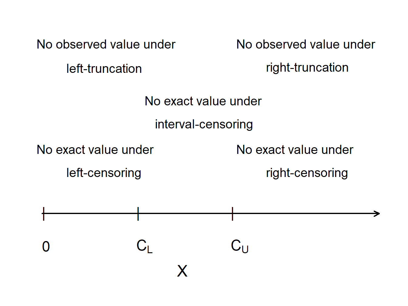
Figure 5.1: Censoring and Truncation

---

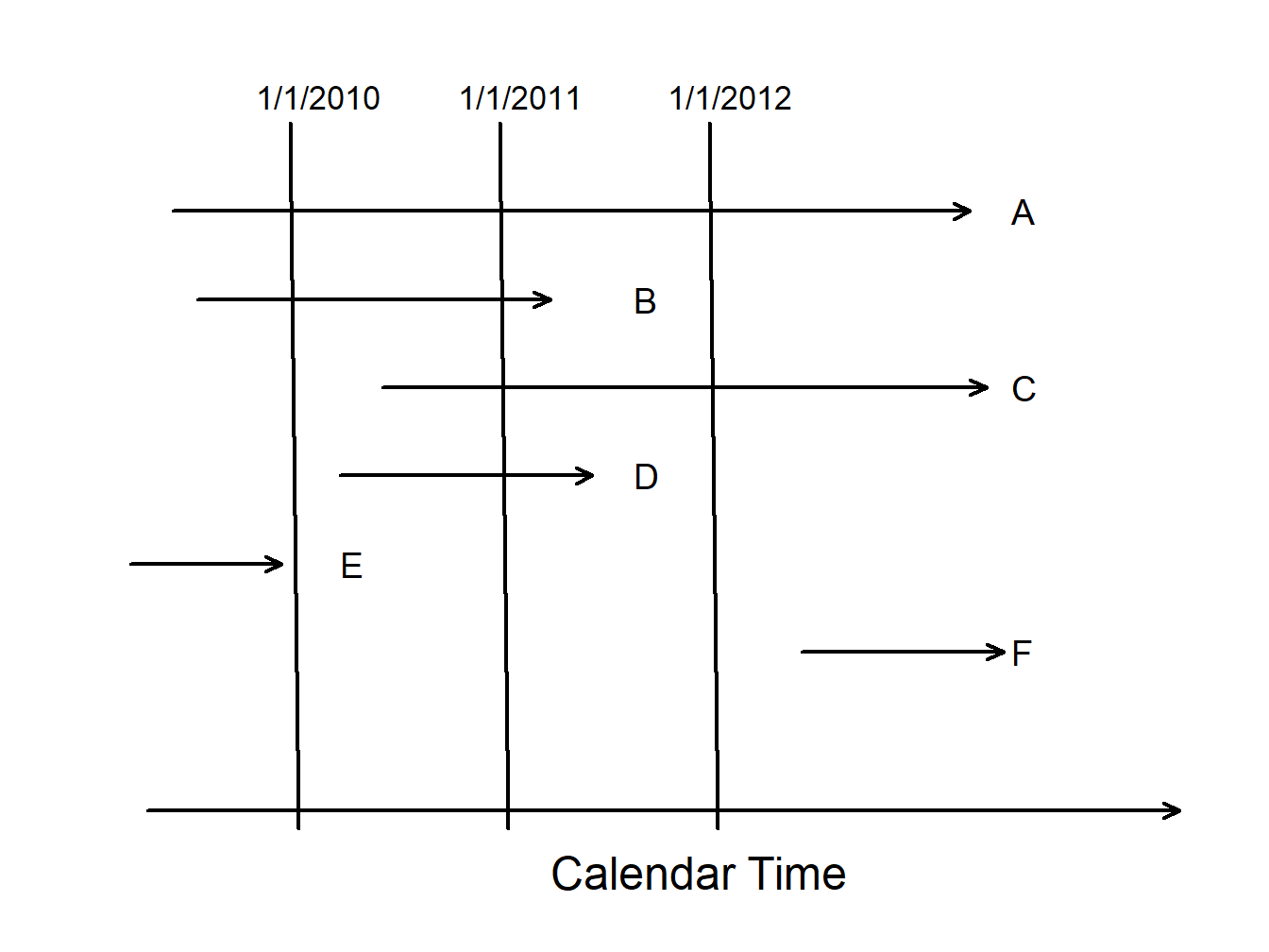
Show Mortality Study Example

Example – Mortality Study. Suppose that you are conducting a two-year study of mortality of high-risk subjects, beginning January 1, 2010 and finishing January 1, 2012. Figure 5.2 graphically portrays the six types of subjects recruited. For each subject, the beginning of the arrow represents that the subject was recruited and the arrow end represents the event time where in this example the event represents death. The arrow represents exposure time.

Figure 5.2: Timeline for Several Subjects on Test in a Mortality Study

• Type A - Right-censored. This subject is alive at the beginning and the end of the study. Because the time of death is not known by the end of the study, it is right-censored. Most subjects are Type A.
• Type B - Complete information is available for a type B subject. The subject is alive at the beginning of the study and the death occurs within the observation period.
• Type C - Right-censored and left-truncated. A type C subject is right-censored, in that death occurs after the observation period. However, the subject entered after the start of the study and is said to have a delayed entry time. Because the subject would not have been observed had death occurred before entry, it is left-truncated.
• Type D - Left-truncated. A type D subject also has delayed entry. Because death occurs within the observation period, this subject is not right censored.
• Type E - Left-truncated. A type E subject is not included in the study because death occurs prior to the observation period.
• Type F - Right-truncated. Similarly, a type F subject is not included because the entry time occurs after the observation period.

---

To summarize, for outcome \(X\) and constants \(C_L\) and \(C_U\),

Limitation Type	Limited Variable	Recording Information
right censoring	\(X_U^{\ast}= \min(X, C_U)\)	\(\delta_U= I(X \le C_U)\)
left censoring	\(X_L^{\ast}= \max(X, C_L)\)	\(\delta_L= I(X > C_L)\)
interval censoring
right truncation	\(X\)	observe \(X\) if \(X \le C_U\)
left truncation	\(X\)	observe \(X\) if \(X > C_L\)

5.2.4 Parametric Estimation using Censored and Truncated Data

For simplicity, we assume non-random censoring amounts and a continuous outcome \(X\). To begin, consider the case of right-censored data where we record \(X_U^{\ast}= \min(X, C_U)\) and censoring indicator \(\delta= I(X \le C_U)\). If censoring occurs so that \(\delta=0\), then \(X > C_U\) and the likelihood is \(\Pr(X > C_U) = 1-F(C_U)\). If censoring does not occur so that \(\delta=1\), then \(X \le C_U\) and the likelihood is \(f(x)\). Summarizing, we have the likelihood of a single observation as

\[ \begin{aligned} \left\{ \begin{array}{ll} 1-F(C_U) & \text{if }\delta=0 \\ f(x) & \text{if } \delta = 1 \end{array} \right. = \left\{ f(x)\right\}^{\delta} \left\{1-F(C_U)\right\}^{1-\delta} . \end{aligned} \]

The right-hand expression allows us to present the likelihood more compactly. Now, for an iid sample of size \(n\), the likelihood is

\[ L(\theta) = \prod_{i=1}^n \left\{ f(x_i)\right\}^{\delta_i} \left\{1-F(C_{Ui})\right\}^{1-\delta_i} = \prod_{\delta_i=1} f(x_i) \prod_{\delta_i=0} \{1-F(C_{Ui})\}, \]

with potential censoring times \(\{ C_{U1}, \ldots,C_{Un} \}\). Here, the notation “\(\prod_{\delta_i=1}\)” means to take the product over uncensored observations, and similarly for “\(\prod_{\delta_i=0}\).”

On the other hand, truncated data are handled in likelihood inference via conditional probabilities. Specifically, we adjust the likelihood contribution by dividing by the probability that the variable was observed. To summarize, we have the following contributions to the likelihood function for six types of outcomes:

\[ {\small \begin{array}{lc} \hline \text{Outcome} & \text{Likelihood Contribution} \\ \hline \text{exact value} & f(x) \\ \text{right-censoring} & 1-F(C_U) \\ \text{left-censoring} & F(C_L) \\ \text{right-truncation} & f(x)/F(C_U) \\ \text{left-truncation} & f(x)/(1-F(C_L)) \\ \text{interval-censoring} & F(C_U)-F(C_L) \\ \hline \end{array} } \]

For known outcomes and censored data, the likelihood is \[L(\theta) = \prod_{E} f(x_i) \prod_{R} \{1-F(C_{Ui})\} \prod_{L} F(C_{Li}) \prod_{I} (F(C_{Ui})-F(C_{Li})),\] where “\(\prod_{E}\)” is the product over observations with Exact values, and similarly for \(R\)ight-, \(L\)eft-
and \(I\)nterval-censoring.

For right-censored and left-truncated data, the likelihood is \[L(\theta) = \prod_{E} \frac{f(x_i)}{1-F(C_{Li})} \prod_{R} \frac{1-F(C_{Ui})}{1-F(C_{Li})},\] and similarly for other combinations. To get further insights, consider the following.

---

Show Special Case - Exponential Distribution

Special Case: Exponential Distribution. Consider data that are right-censored and left-truncated, with random variables \(X_i\) that are exponentially distributed with mean \(\theta\). With these specifications, recall that \(f(x) = \theta^{-1} \exp(-x/\theta)\) and \(F(x) = 1-\exp(-x/\theta)\).

For this special case, the log-likelihood is

\[ \begin{aligned} l(\theta) &= \sum_{E} \left\{ \log f(x_i) - \log (1-F(C_{Li})) \right\} + \sum_{R}\left\{ \log (1-F(C_{Ui}))- \log (1-\mathrm{F}(C_{Li})) \right\}\\ &= \sum_{E} (-\log \theta -(x_i-C_{Li})/\theta ) -\sum_{R} (C_{Ui}-C_{Li})/\theta . \end{aligned} \]

To simplify the notation, define \(\delta_i = I(X_i < C_{Ui})\) to be a binary variable that indicates right-censoring. Let \(X_i^{\ast \ast} = \min(X_i, C_{Ui}) - C_{Li}\) be the amount that the observed variable exceeds the lower truncation limit. With this, the log-likelihood is

\[\begin{equation} l(\theta) = - \sum_{i=1}^n \left((1-\delta_i) \log \theta + \frac{x_i^{\ast \ast}}{\theta}\right) \tag{5.1} \end{equation}\]

Taking derivatives with respect to the parameter \(\theta\) and setting it equal to zero yields the maximum likelihood estimator

\[ \widehat{\theta} = \frac{1}{n_u} \sum_{i=1}^n x_i^{\ast \ast}, \]

where \(n_u = \sum_i (1-\delta_i)\) is the number of uncensored observations.

---

Example 5.2.2. Actuarial Exam Question. You are given:

1. A sample of losses is: 600 700 900
2. No information is available about losses of 500 or less.
3. Losses are assumed to follow an exponential distribution with mean \(\theta\).

Calculate the maximum likelihood estimate of \(\theta\).

Show Example Solution

Solution. These observations are truncated at 500. The contribution of each observation to the likelihood function is \[\frac{f(x)}{1-F(500)} = \frac{\theta^{-1}e^{-x/\theta}}{e^{-500/\theta}}\]

Then the likelihood function is

\[L(\theta)= \frac{\theta^{-1} e^{-600/\theta} \theta^{-1} e^{-700/\theta} \theta^{-1} e^{-900/\theta}}{(e^{-500/\theta})^3} = \theta^{-3}e^{-700/\theta}\]

The log-likelihood is

\[ l(\theta) = \log L(\theta) = -3 \log \theta - 700 \theta^{-1} \]

Maximizing this expression by setting the derivative with respect to \(\theta\) equal to 0, we have

\[ L'(\theta) = -3 \theta^{-1} + 700 \theta^{-2} = 0 \ \Rightarrow \ \hat{\theta} = \frac{700}{3} = 233.33 . \]

---

Example 5.2.3. Actuarial Exam Question. You are given the following information about a random sample:

1. The sample size equals five.
2. The sample is from a Weibull distribution with \(\tau=2\).
3. Two of the sample observations are known to exceed 50, and the remaining three observations are 20, 30, and 45.

Calculate the maximum likelihood estimate of \(\theta\).

Show Example Solution

Solution. The likelihood function is

\[ \begin{aligned} L(\theta) &= f(20) f(30) f(45) [1-F(50)]^2 \\ &= \frac{2(20/\theta)^2 e^{-(20/\theta)^2}}{20} \frac{2(30/\theta)^2 e^{-(30/\theta)^2}}{30} \frac{2(45/\theta)^2 e^{-(45/\theta)^2}}{45}(e^{-(50/\theta)^2})^2 \\ &\propto \frac{1}{\theta^6} e^{-8325/\theta^2} \end{aligned} \]

The natural logarithm of the above expression is \(-6\log\theta - \frac{8325}{\theta^2}\). Maximizing this expression by setting its derivative to 0, we get

\[\frac{-6}{\theta} + \frac{16650}{\theta^3} = 0 \ \Rightarrow \ \hat{\theta} = \left(\frac{16650}{6}\right)^{\frac{1}{2}} = 52.6783\]

---

5.3 Nonparametric Estimation using Modified Data

---

In this section, you learn how to:

• Estimate the distribution function for grouped data using the ogive.
• Create a nonparametric estimator of the loss elimination ratio using the plug-in principle.
• Apply the Kaplan-Meier product-limit and the Nelson Aalon estimators to estimate the distribution function in the presence of censoring.
• Apply Greenwood’s formula to estimate the variance of the product-limit estimator.

---

Nonparametric estimators provide useful benchmarks, so it is helpful to understand the estimation procedures for grouped, censored, and truncated data.

5.3.1 Grouped Data

As we have seen in Section 5.2.1, observations may be grouped (also referred to as interval censored) in the sense that we only observe them as belonging in one of \(k\) intervals of the form \((c_{j-1}, c_j]\), for \(j=1, \ldots, k\). At the boundaries, the empirical distribution function is defined in the usual way: \[ F_n(c_j) = \frac{\text{number of observations } \le c_j}{n}. \]

Ogive Estimator. For other values of \(x \in (c_{j-1}, c_j)\), we can estimate the distribution function with the ogive estimatorA nonparametric estimator for the distribution function in the presence of grouped data., which linearly interpolates between \(F_n(c_{j-1})\) and \(F_n(c_j)\), i.e. the values of the boundaries \(F_n(c_{j-1})\) and \(F_n(c_j)\) are connected with a straight line. This can formally be expressed as \[F_n(x) = \frac{c_j-x}{c_j-c_{j-1}} F_n(c_{j-1}) + \frac{x-c_{j-1}}{c_j-c_{j-1}} F_n(c_j) \ \ \ \text{for } c_{j-1} \le x < c_j\]

The corresponding density is

\[ f_n(x) = F^{\prime}_n(x) = \frac{F_n(c_j)-F_n(c_{j-1})}{c_j - c_{j-1}} \ \ \ \text{for } c_{j-1} < x < c_j . \]

---

Example 5.3.1. Actuarial Exam Question. You are given the following information regarding claim sizes for 100 claims:

\[ {\small \begin{array}{r|c} \hline \text{Claim Size} & \text{Number of Claims} \\ \hline 0 - 1,000 & 16 \\ 1,000 - 3,000 & 22 \\ 3,000 - 5,000 & 25 \\ 5,000 - 10,000 & 18 \\ 10,000 - 25,000 & 10 \\ 25,000 - 50,000 & 5 \\ 50,000 - 100,000 & 3 \\ \text{over } 100,000 & 1 \\ \hline \end{array} } \]

Using the ogive, calculate the estimate of the probability that a randomly chosen claim is between 2000 and 6000.

Show Example Solution

Solution. At the boundaries, the empirical distribution function is defined in the usual way, so we have \[F_{100}(1000) = 0.16, \ F_{100}(3000)=0.38, \ F_{100}(5000)=0.63, \ F_{100}(10000)=0.81\] For other claim sizes, the ogive estimator linearly interpolates between these values:

\[ \begin{array}{ll} F_{100}(2000) &= 0.5F_{100}(1000) + 0.5F_{100}(3000) = 0.5(0.16)+0.5(0.38)=0.27 \\ F_{100}(6000) &=0.8F_{100}(5000)+0.2F_{100}(10000) = 0.8(0.63)+0.2(0.81)=0.666 \end{array} \]

Thus, the probability that a claim is between 2000 and 6000 is \(F_{100}(6000) - F_{100}(2000) = 0.666-0.27 = 0.396\).

---

5.3.2 Plug-in Principle

One way to create a nonparametric estimator of some quantity is to use the analog or plug-in principleThe plug-in principle or analog principle of estimation proposes that population parameters be estimated by sample statistics which have the same property in the sample as the parameters do in the population. where one replaces the unknown cdfCumulative distribution function \(F\) with a known estimate such as the empirical cdf \(F_n\). So, if we are trying to estimate \(\mathrm{E}~[\mathrm{g}(X)]=\mathrm{E}_F~[\mathrm{g}(X)]\) for a generic function g, then we define a nonparametric estimator to be \(\mathrm{E}_{F_n}~[\mathrm{g}(X)]=n^{-1}\sum_{i=1}^n \mathrm{g}(X_i)\).

To see how this works, as a special case of g we consider the loss per payment random variable is \(Y = (X-d)_+\) and the loss elimination ratio introduced in Section 4.4.1. We can express this as \[ LER(d) = \frac{\mathrm{E~}[X - (X-d)_+]}{\mathrm{E~}[X]} =\frac{\mathrm{E~}[\min(X,d)]}{\mathrm{E~}[X]} , \] for a fixed deductible \(d\).

Example. 5.3.2. Bodily Injury Claims and Loss Elimination Ratios

We use a sample of 432 closed auto claims from Boston from Derrig, Ostaszewski, and Rempala (2001). Losses are recorded for payments due to bodily injuries in auto accidents. Losses are not subject to deductibles but are limited by various maximum coverage amounts that are also available in the data. It turns out that only 17 out of 432 (\(\approx\) 4%) were subject to these policy limits and so we ignore these data for this illustration.

The average loss paid is 6906 in U.S. dollars. Figure 5.3 shows other aspects of the distribution. Specifically, the left-hand panel shows the empirical distribution function, the right-hand panel gives a nonparametric density plot.

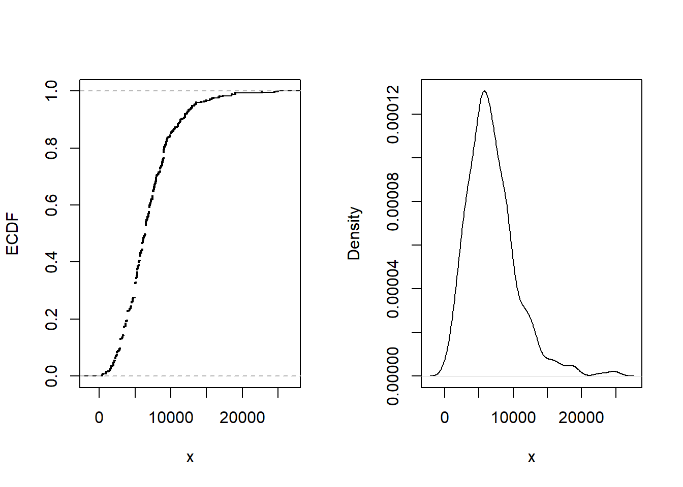
Figure 5.3: Bodily Injury Claims. The left-hand panel gives the empirical distribution function. The right-hand panel presents a nonparametric density plot.

The impact of bodily injury losses can be mitigated by the imposition of limits or purchasing reinsurance policies (see Section 10.3). To quantify the impact of these risk mitigation tools, it is common to compute the loss elimination ratio (LER) as introduced in Section 4.4.1. The distribution function is not available and so must be estimated in some way. Using the plug-in principle, a nonparametric estimator can be defined as

\[ LER_n(d) = \frac{n^{-1} \sum_{i=1}^n \min(X_i,d)}{n^{-1} \sum_{i=1}^n X_i} = \frac{\sum_{i=1}^n \min(X_i,d)}{\sum_{i=1}^n X_i} . \]

Figure 5.4 shows the estimator \(LER_n(d)\) for various choices of \(d\). For example, at \(d=1,000\), we have \(LER_n(1000) \approx\) 0.1442. Thus, imposing a limit of 1,000 means that expected retained claims are 14.42 percent lower when compared to expected claims with a zero deductible.

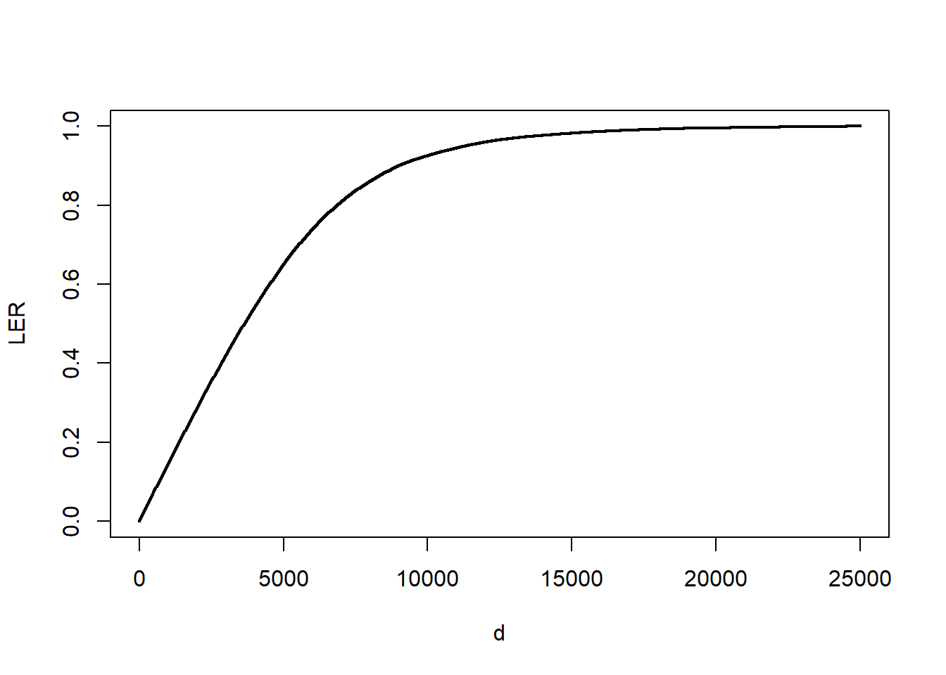
Figure 5.4: LER for Bodily Injury Claims. The figure presents the loss elimination ratio (LER) as a function of deductible \(d\).

5.3.3 Right-Censored Empirical Distribution Function

It can be useful to calibrate parametric estimators with nonparametric methods that do not rely on a parametric form of the distribution. The product-limit estimatorA nonparametric estimator of the survival function in the presence of incomplete data. also known as the kaplan-meier estimator. due to (Kaplan and Meier 1958) is a well-known estimator of the distribution function in the presence of censoring.

Motivation for the Kaplan-Meier Product Limit Estimator. To explain why the product-limit works so well with censored observations, let us first return to the “usual” case without censoring. Here, the empirical distribution function \(F_n(x)\) is an unbiased estimator of the distribution function \(F(x)\). This is because \(F_n(x)\) is the average of indicator variables each of which are unbiased, that is, \(\mathrm{E~} [I(X_i \le x)] = \Pr(X_i \le x) = F(x)\).

Now suppose the random outcome is censored on the right by a limiting amount, say, \(C_U\), so that we record the smaller of the two, \(X^* = \min(X, C_U)\). For values of \(x\) that are smaller than \(C_U\), the indicator variable still provides an unbiased estimator of the distribution function before we reach the censoring limit. That is, \(\mathrm{E~} [I(X^* \le x)] = F(x)\) because \(I(X^* \le x) = I(X \le x)\) for \(x < C_U\). In the same way, \(\mathrm{E~} [I(X^* > x)] = 1 -F(x) = S(x)\). But, for \(x>C_U\), \(I(X^* \le x)\) is in general not an unbiased estimator of \(F(x)\).

As an alternative, consider two random variables that have different censoring limits. For illustration, suppose that we observe \(X_1^* = \min(X_1, 5)\) and \(X_2^* = \min(X_2, 10)\) where \(X_1\) and \(X_2\) are independent draws from the same distribution. For \(x \le 5\), the empirical distribution function \(F_2(x)\) is an unbiased estimator of \(F(x)\). However, for \(5 < x \le 10\), the first observation cannot be used for the distribution function because of the censoring limitation. Instead, the strategy developed by (Kaplan and Meier 1958) is to use \(S_2(5)\) as an estimator of \(S(5)\) and then to use the second observation to estimate the survival function conditional on survival to time 5, \(\Pr(X > x | X >5) = \frac{S(x)}{S(5)}\). Specifically, for \(5 < x \le 10\), the estimator of the survival function is

\[ \hat{S}(x) = S_2(5) \times I(X_2^* > x ) . \]

Kaplan-Meier Product Limit Estimator. Extending this idea, for each observation \(i\), let \(u_i\) be the upper censoring limit (\(=\infty\) if no censoring). Thus, the recorded value is \(x_i\) in the case of no censoring and \(u_i\) if there is censoring. Let \(t_{1} <\cdots< t_{k}\) be \(k\) distinct points at which an uncensored loss occurs, and let \(s_j\) be the number of uncensored losses \(x_i\)’s at \(t_{j}\). The corresponding risk setThe number of observations that are active (not censored) at a specific point. is the number of observations that are active (not censored) at a value less than \(t_{j}\), denoted as \(R_j = \sum_{i=1}^n I(x_i \geq t_{j}) + \sum_{i=1}^n I(u_i \geq t_{j})\).

With this notation, the product-limit estimator of the distribution function is

\[\begin{equation} \hat{F}(x) = \left\{ \begin{array}{ll} 0 & x<t_{1} \\ 1-\prod_{j:t_{j} \leq x}\left( 1-\frac{s_j}{R_{j}}\right) & x \geq t_{1} \end{array} \right. . \tag{5.2} \end{equation}\]

For example, if \(x\) is smaller than the smallest uncensored loss, then \(x<t_1\) and \(\hat{F}(x) =0\). As another example, if \(x\) falls between then second and third smallest uncensored losses, then \(x \in (t_2,t_3]\) and \(\hat{F}(x) = 1 - \left(1- \frac{s_1}{R_{1}}\right)\left(1- \frac{s_2}{R_{2}}\right)\).

As usual, the corresponding estimate of the survival function is \(\hat{S}(x) = 1 - \hat{F}(x)\).

---

Example 5.3.3. Actuarial Exam Question. The following is a sample of 10 payments:

\[ \begin{array}{cccccccccc} 4 &4 &5+ &5+ &5+ &8 &10+ &10+ &12 &15 \\ \end{array} \]

where \(+\) indicates that a loss has exceeded the policy limit.

Using the Kaplan-Meier product-limit estimator, calculate the probability that the loss on a policy exceeds 11, \(\hat{S}(11)\).

Show Example Solution

Solution. There are four event times (non-censored observations). For each time \(t_j\), we can calculate the number of events \(s_j\) and the risk set \(R_j\) as the following:

\[ \begin{array}{cccc} \hline j & t_j & s_j & R_j \\ \hline 1 & 4 & 2 & 10 \\ 2 & 8 & 1 & 5 \\ 3 & 12 & 1 & 2 \\ 4 & 15 & 1 & 1 \\ \hline \end{array} \]

Thus, the Kaplan-Meier estimate of \(S(11)\) is \[ \begin{aligned} \hat{S}(11) &= \prod_{j:t_j\leq 11} \left( 1- \frac{s_j}{R_j} \right) = \prod_{j=1}^{2} \left( 1- \frac{s_j}{R_j} \right)\\ &= \left(1-\frac{2}{10} \right) \left(1-\frac{1}{5} \right) = (0.8)(0.8)= 0.64. \\ \end{aligned} \]

---

Example. 5.3.4. Bodily Injury Claims. We consider again the Boston auto bodily injury claims data from Derrig, Ostaszewski, and Rempala (2001) that was introduced in Example 5.1.11. In that example, we omitted the 17 claims that were censored by policy limits. Now, we include the full dataset and use the Kaplan-Meier product limit to estimate the survival function. This is given in Figure 5.5.

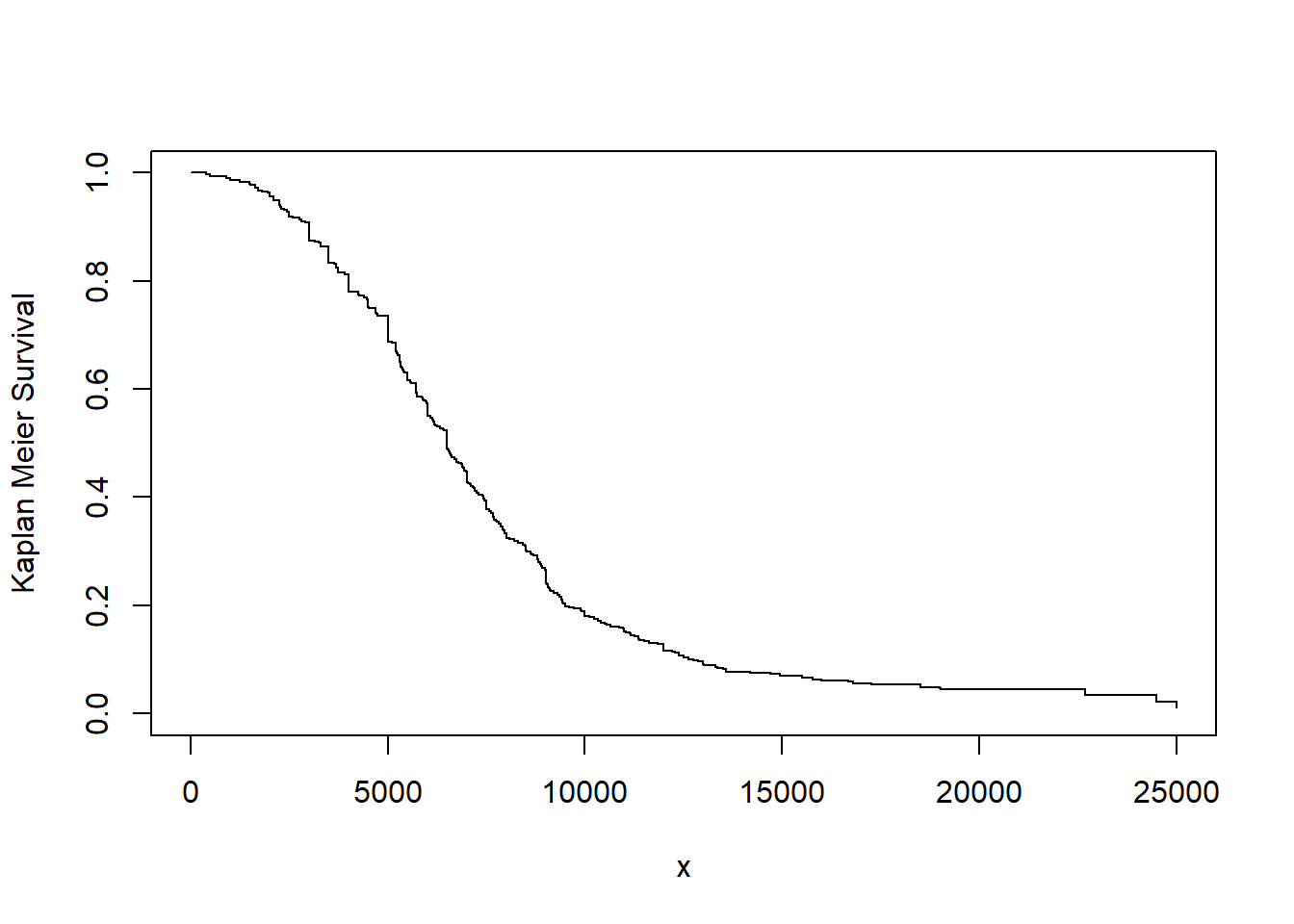
Figure 5.5: Kaplan-Meier Estimate of the Survival Function for Bodily Injury Claims

Show R Code

library(survival)  # for Surv(), survfit()
# BIData <- read.csv('Data/DerrigResampling.csv', header =T)
BIData$UnCensored <- 1 * (BIData$AmountPaid < BIData$PolicyLimit)
## KM estimate
KM0 <- survfit(Surv(AmountPaid, UnCensored) ~ 1, type = "kaplan-meier", data = BIData)
plot(KM0, conf.int = FALSE, xlab = "x", ylab = "Kaplan Meier Survival")

---

Right-Censored, Left-Truncated Empirical Distribution Function. In addition to right-censoring, we now extend the framework to allow for left-truncated data. As before, for each observation \(i\), let \(u_i\) be the upper censoring limit (\(=\infty\) if no censoring). Further, let \(d_i\) be the lower truncation limit (0 if no truncation). Thus, the recorded value (if it is greater than \(d_i\)) is \(x_i\) in the case of no censoring and \(u_i\) if there is censoring. Let \(t_{1} <\cdots< t_{k}\) be \(k\) distinct points at which an event of interest occurs, and let \(s_j\) be the number of recorded events \(x_i\)’s at time point \(t_{j}\). The corresponding risk set is \[R_j = \sum_{i=1}^n I(x_i \geq t_{j}) + \sum_{i=1}^n I(u_i \geq t_{j}) - \sum_{i=1}^n I(d_i \geq t_{j}).\]

With this new definition of the risk set, the product-limit estimator of the distribution function is as in equation (5.2).

Greenwood’s Formula. (Greenwood 1926) derived the formula for the estimated variance of the product-limit estimator to be

\[ \widehat{Var}(\hat{F}(x)) = (1-\hat{F}(x))^{2} \sum _{j:t_{j} \leq x} \dfrac{s_j}{R_{j}(R_{j}-s_j)}. \]

As usual, we refer to the square root of the estimated variance as a standard error, a quantity that is routinely used in confidence intervals and for hypothesis testing. To compute this, R‘s survfit method takes a survival data object and creates a new object containing the Kaplan-Meier estimate of the survival function along with confidence intervals. The Kaplan-Meier method (type='kaplan-meier') is used by default to construct an estimate of the survival curve. The resulting discrete survival function has point masses at the observed event times (discharge dates) \(t_j\), where the probability of an event given survival to that duration is estimated as the number of observed events at the duration \(s_j\) divided by the number of subjects exposed or ’at-risk’ just prior to the event duration \(R_j\).

Alternative Estimators. Two alternate types of estimation are also available for the survfit method. The alternative (type='fh2') handles ties, in essence, by assuming that multiple events at the same duration occur in some arbitrary order. Another alternative (type='fleming-harrington') uses the Nelson-AalenA nonparametric estimator of the cumulative hazard function in the presence of incomplete data. (see (Aalen 1978)) estimate of the cumulative hazard function to obtain an estimate of the survival function. The estimated cumulative hazard \(\hat{H}(x)\) starts at zero and is incremented at each observed event duration \(t_j\) by the number of events \(s_j\) divided by the number at risk \(R_j\). With the same notation as above, the Nelson-Äalen estimator of the distribution function is

\[ \begin{aligned} \hat{F}_{NA}(x) &= \left\{ \begin{array}{ll} 0 & x<t_{1} \\ 1- \exp \left(-\sum_{j:t_{j} \leq x}\frac{s_j}{R_j} \right) & x \geq t_{1} \end{array} \right. .\end{aligned} \]

Note that the above expression is a result of the Nelson-Äalen estimator of the cumulative hazard function \[\hat{H}(x)=\sum_{j:t_j\leq x} \frac{s_j}{R_j} \] and the relationship between the survival function and cumulative hazard function, \(\hat{S}_{NA}(x)=e^{-\hat{H}(x)}\).

---

Example 5.3.5. Actuarial Exam Question.

For observation \(i\) of a survival study:

• \(d_i\) is the left truncation point
• \(x_i\) is the observed value if not right censored
• \(u_i\) is the observed value if right censored

You are given:

\[ {\small \begin{array}{c|cccccccccc} \hline \text{Observation } (i) & 1 & 2 & 3 & 4 & 5 & 6 & 7 & 8 & 9 & 10\\ \hline d_i & 0 & 0 & 0 & 0 & 0 & 0 & 0 & 1.3 & 1.5 & 1.6\\ x_i & 0.9 & - & 1.5 & - & - & 1.7 & - & 2.1 & 2.1 & - \\ u_i & - & 1.2 & - & 1.5 & 1.6 & - & 1.7 & - & - & 2.3 \\ \hline \end{array} } \]

Calculate the Kaplan-Meier product-limit estimate, \(\hat{S}(1.6)\)

Show Example Solution

Solution. Recall the risk set \(R_j = \sum_{i=1}^n \left\{ I(x_i \geq t_{j}) + I(u_i \geq t_{j}) - I(d_i \geq t_{j}) \right\}\). Then

\[ \begin{array}{ccccc} \hline j & t_j & s_j & R_j & \hat{S}(t_j) \\ \hline 1 & 0.9 & 1 & 10-3 = 7 & 1-\frac{1}{7} = \frac{6}{7} \\ 2 & 1.5 & 1 & 8-2 = 6 & \frac{6}{7}\left( 1 - \frac{1}{6} \right) = \frac{5}{7}\\ 3 & 1.7 & 1 & 5-0 = 5 & \frac{5}{7}\left( 1 - \frac{1}{5} \right) = \frac{4}{7}\\ 4 & 2.1 & 2 & 3 & \frac{4}{7}\left( 1 - \frac{2}{3}\right) = \frac{4}{21}\\ \hline \end{array} \]

The Kaplan-Meier estimate is therefore \(\hat{S}(1.6) = \frac{5}{7}\).

---

Example 5.3.6. Actuarial Exam Question. - Continued.

1. Using the Nelson-Äalen estimator, calculate the probability that the loss on a policy exceeds 11, \(\hat{S}_{NA}(11)\).
2. Calculate Greenwood’s approximation to the variance of the product-limit estimate \(\hat{S}(11)\).

Show Example Solution

Solution. As before, there are four event times (non-censored observations). For each time \(t_j\), we can calculate the number of events \(s_j\) and the risk set \(R_j\) as the following:

\[ \begin{array}{cccc} \hline j & t_j & s_j & R_j \\ \hline 1 & 4 & 2 & 10 \\ 2 & 8 & 1 & 5 \\ 3 & 12 & 1 & 2 \\ 4 & 15 & 1 & 1 \\ \hline \end{array} \]

The Nelson-Äalen estimate of \(S(11)\) is \(\hat{S}_{NA}(11)=e^{-\hat{H}(11)} = e^{-0.4} = 0.67\), since \[ \begin{aligned} \hat{H}(11) &= \sum_{j:t_j\leq 11} \frac{s_j}{R_j} = \sum_{j=1}^{2} \frac{s_j}{R_j} \\ &= \frac{2}{10} + \frac{1}{5} = 0.2 + 0.2 = 0.4 .\\ \end{aligned} \]

From earlier work, the Kaplan-Meier estimate of \(S(11)\) is \(\hat{S}(11) = 0.64\). Then Greenwood’s estimate of the variance of the product-limit estimate of \(S(11)\) is \[ \begin{aligned} \widehat{Var}(\hat{S}(11)) &= (\hat{S}(11))^2 \sum_{j:t_j\leq 11} \frac{s_j}{R_j(R_j-s_j)} &= (0.64)^2 \left(\frac{2}{10(8)} + \frac{1}{5(4)} \right) = 0.0307. \\ \end{aligned} \]

---

Show Quiz Solution

---

5.4 Further Resources and Contributors

Exercises

Here are a set of exercises that guide the viewer through some of the theoretical foundations of Loss Data Analytics. Each tutorial is based on one or more questions from the professional actuarial examinations, typically the Society of Actuaries Exam C/STAM.

Model Selection Guided Tutorials

Contributors

• Zeinab Amin, The American University in Cairo, is the principal author of this chapter. Email: zeinabha@aucegypt.edu for chapter comments and suggested improvements.
• Edward W. (Jed) Frees and Lisa Gao, University of Wisconsin-Madison, are the principal authors of the sections on estimation using modified data which appeared in chapter 4 of the first edition of the text.
  
• Chapter reviewers include: Vytaras Brazauskas, Yvonne Chueh, Eren Dodd, Hirokazu (Iwahiro) Iwasawa, Joseph Kim, Andrew Kwon-Nakamura, Jiandong Ren, and Di (Cindy) Xu.

Bibliography

Aalen, Odd. 1978. “Nonparametric Inference for a Family of Counting Processes.” The Annals of Statistics 6 (4): 701–26.

Derrig, Richard A, Krzysztof M Ostaszewski, and Grzegorz A Rempala. 2001. “Applications of Resampling Methods in Actuarial Practice.” In Proceedings of the Casualty Actuarial Society, 87:322–64. Casualty Actuarial Society.

Greenwood, Major. 1926. “The Errors of Sampling of the Survivorship Tables.” In Reports on Public Health and Statistical Subjects. Vol. 33. London: Her Majesty’s Stationary Office.

Kaplan, Edward L., and Paul Meier. 1958. “Nonparametric Estimation from Incomplete Observations.” Journal of the American Statistical Association 53 (282): 457–81.